Experimental Design and Analysis Assessment 1 (Autumn Semester 2019)
VerifiedAdded on 2022/11/14
|19
|5249
|287
AI Summary
This document contains three scenarios for Experimental Design and Analysis Assessment 1 (Autumn Semester 2019) with statistical analysis and results. The scenarios include determining the cleanliness attitudes of employees, the effectiveness of a weight-gain program, and the productivity of workers in a factory.
Contribute Materials
Your contribution can guide someone’s learning journey. Share your
documents today.
Experimental Design and Analysis 100013 –Autumn 2019
Assessment 1 (Autumn Semester 2019)
Scenario 1
A large food manufacturing company seeks to determine the cleanliness attitudes of their
250 employees, compared to the general population. You are tasked to compare the
cleanliness attitudes of a sample of employees with the population cleanliness attitude.
You measure employees’ responses using the Happiness at Work Scale, which validly
measures work happiness. This scale provides a number from 1 to 50, wher
e 1 refers to very low happiness, and 50 signifies extreme happiness. The population
mean for “work happiness” on this scale is 25, but you don’t have access to the
population standard deviation.
Your analysis will examine happiness differences between the company employees and
the population. You predict the employees will show a higher work happiness score than
the population.
You randomly recruit 30 employees from the 250, and they all agree to complete the
Happiness at Work Scale at the organisation’s head office on a Friday morning. The data
you collect from the 30 participants is shown in Table 1.
Task 1
(1) Write a results section (“draft answer”). 1 mark for this “working out”
Hypothesis Testing:
Null hypothesis (Ho): Company employees had no significant difference in happiness
scores compared to the population.
Alternative hypothesis (H1): Employees have a higher work happiness score than the
population.
(2) What is the name of the statistical analysis you used? 1 mark
One-Sample t-test .This was necessary for comparing means for a small sample
(3) What is the mean age of male and female participants? 1 mark
Female = X = ∑ X
N = 547
17 =32.18
Male = X = ∑ X
N = 407
13 =31.31
1
Secure Best Marks with AI Grader
Need help grading? Try our AI Grader for instant feedback on your assignments.
Experimental Design and Analysis 100013 –Autumn 2019
(4) Which (if any) participant was an outlier? (Provide their ID number, or write “no
outlier” if you didn’t identify anyone). 1 mark
The happiness scores had an outlier
ID NO:29
(5) If there was an outlier, what number did you change their score to? (write “Not
applicable” if there was no outlier). 1 mark
The happiness score range from 35 to 50.This could have been a typing error when
imputing the data. I changed this from 2 to 42.
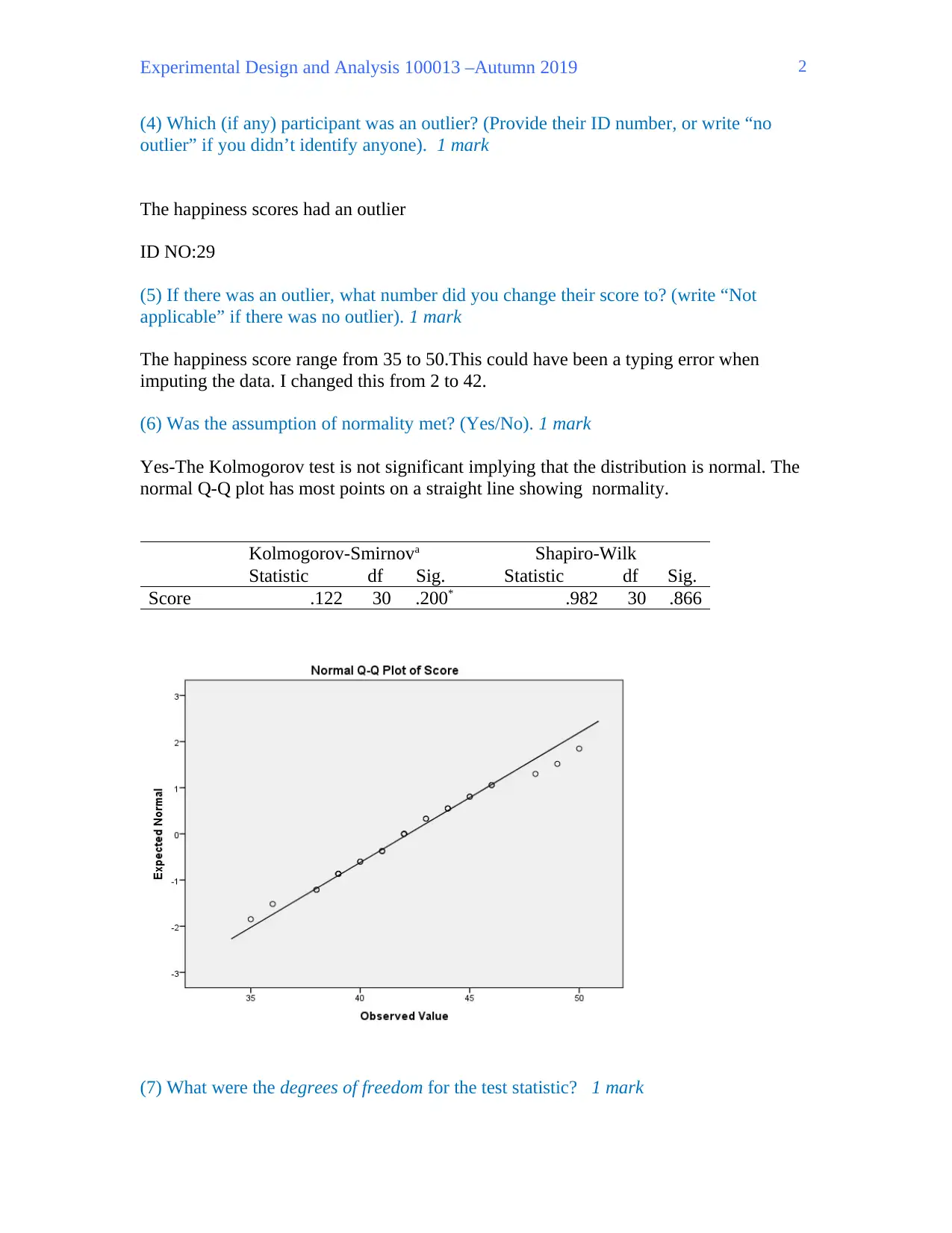
(6) Was the assumption of normality met? (Yes/No). 1 mark
Yes-The Kolmogorov test is not significant implying that the distribution is normal. The
normal Q-Q plot has most points on a straight line showing normality.
Kolmogorov-Smirnova Shapiro-Wilk
Statistic df Sig. Statistic df Sig.
Score .122 30 .200* .982 30 .866
(7) What were the degrees of freedom for the test statistic? 1 mark
2
(4) Which (if any) participant was an outlier? (Provide their ID number, or write “no
outlier” if you didn’t identify anyone). 1 mark
The happiness scores had an outlier
ID NO:29
(5) If there was an outlier, what number did you change their score to? (write “Not
applicable” if there was no outlier). 1 mark
The happiness score range from 35 to 50.This could have been a typing error when
imputing the data. I changed this from 2 to 42.
(6) Was the assumption of normality met? (Yes/No). 1 mark
Yes-The Kolmogorov test is not significant implying that the distribution is normal. The
normal Q-Q plot has most points on a straight line showing normality.
Kolmogorov-Smirnova Shapiro-Wilk
Statistic df Sig. Statistic df Sig.
Score .122 30 .200* .982 30 .866
(7) What were the degrees of freedom for the test statistic? 1 mark
2
Experimental Design and Analysis 100013 –Autumn 2019
d.f =n-1= 29
(8) What was the value of the test statistic? 1 mark
Test Value = 0
t
d
f
Sig.
(2-
taile
d)
Mean
Differen
ce
95%
Confidence
Interval of
the
Difference
Low
er
Upp
er
Scor
e
64.992 2
9
.000 42.200 40.8
7
43.5
3
Test statistic t =64.99
(9) What was the probability value associated with the test statistic? (use “p < 0.001” if
the SPSS output shows “0.000” in the probability box). 1 mark
Probability value :p < 0.001
(10) What was the value of the Cohen’s d effect size? (write “Not applicable” if effect
size is not relevant to the Scenario 1 analysis). 1 mark
Since this is not grouped then the cohen d effect size was not considered applicable.
(11) Based on the value of Cohen’s d you might have calculated, how would you describe
the effect size? (small, medium, large or “not applicable”). 1 mark
Since this is not grouped then the cohen d effect size with not be applicable.
TASK 2
Circle the number next to the statement which most accurately summarises the research
findings. 2 marks
(1) The mean happiness rating of the sample was significantly higher than the population
mean.
3
Experimental Design and Analysis 100013 –Autumn 2019
TASK 3
You’ve mistakenly allowed a single, obvious design flaw to potentially affect the validity
of your results. What is it? (only write a single word, phrase or short sentence; for
example, “lack of reliability” or “experimenter effect”). 2 marks
Lack of reliability and validity
Scenario 2
A health-food company is planning to advertise their (new) twelve-day weight-gain
program to the public. The company executives believe the program will be effective in
helping people who have lost weight (due to various chronic illnesses) gain a healthy and
sustainable weight in a short period of time. However, the company requires scientific
evidence that the program is successful, if they are to proceed with the marketing plan.
To help them gather this evidence, you compile a list of 177 patients who have been
identified by medical professionals as having lost significant weight through disease
(which is in remission). You contact these patients and ask them whether they’d be
interested in participating in your study, and if they agree they are to meet you in the
company’s training room on Friday morning so you can measure their weight (kg) and
provide them with the diet program. This program consists of 36 pre-packaged meals
that participants self-administer during the course of the study.
35 participants turn up to your meeting, and after weighing them you explain that the
program consists of eating three of the pre-packaged meals a day; morning, noon and
evening for 12 days. They cannot eat anything else (to ensure control of meal portion
sizes).
All 35 participants begin the program on Monday, which you label Monday Week 1. The
diet regime ends on the Friday of Week 2 (12 consecutive days x 3 meals a day = 36 pre-
packaged meals). All the patients are very enthusiastic and keep a diet diary for the
fortnight, and you later determine that they all correctly followed instructions and ate all
the meals as specified.
On the first Saturday morning after the twelve-day program ends (“Day 13”) you have a
return meeting with the participants in the training room and measure their weight a
second time. You now analyse the data from these participants to answer the company’s
question – did the program result in a significant increase in mean weight for the
participant group?
4
Secure Best Marks with AI Grader
Need help grading? Try our AI Grader for instant feedback on your assignments.
Experimental Design and Analysis 100013 –Autumn 2019
TASK 1
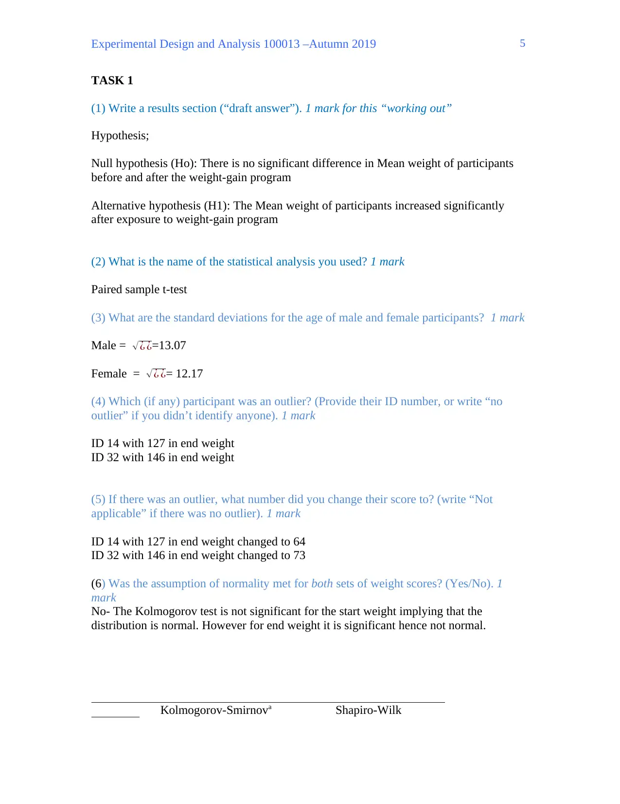
(1) Write a results section (“draft answer”). 1 mark for this “working out”
Hypothesis;
Null hypothesis (Ho): There is no significant difference in Mean weight of participants
before and after the weight-gain program
Alternative hypothesis (H1): The Mean weight of participants increased significantly
after exposure to weight-gain program
(2) What is the name of the statistical analysis you used? 1 mark
Paired sample t-test
(3) What are the standard deviations for the age of male and female participants? 1 mark
Male = √¿ ¿=13.07
Female = √¿ ¿= 12.17
(4) Which (if any) participant was an outlier? (Provide their ID number, or write “no
outlier” if you didn’t identify anyone). 1 mark
ID 14 with 127 in end weight
ID 32 with 146 in end weight
(5) If there was an outlier, what number did you change their score to? (write “Not
applicable” if there was no outlier). 1 mark
ID 14 with 127 in end weight changed to 64
ID 32 with 146 in end weight changed to 73
(6) Was the assumption of normality met for both sets of weight scores? (Yes/No). 1
mark
No- The Kolmogorov test is not significant for the start weight implying that the
distribution is normal. However for end weight it is significant hence not normal.
Kolmogorov-Smirnova Shapiro-Wilk
5
TASK 1
(1) Write a results section (“draft answer”). 1 mark for this “working out”
Hypothesis;
Null hypothesis (Ho): There is no significant difference in Mean weight of participants
before and after the weight-gain program
Alternative hypothesis (H1): The Mean weight of participants increased significantly
after exposure to weight-gain program
(2) What is the name of the statistical analysis you used? 1 mark
Paired sample t-test
(3) What are the standard deviations for the age of male and female participants? 1 mark
Male = √¿ ¿=13.07
Female = √¿ ¿= 12.17
(4) Which (if any) participant was an outlier? (Provide their ID number, or write “no
outlier” if you didn’t identify anyone). 1 mark
ID 14 with 127 in end weight
ID 32 with 146 in end weight
(5) If there was an outlier, what number did you change their score to? (write “Not
applicable” if there was no outlier). 1 mark
ID 14 with 127 in end weight changed to 64
ID 32 with 146 in end weight changed to 73
(6) Was the assumption of normality met for both sets of weight scores? (Yes/No). 1
mark
No- The Kolmogorov test is not significant for the start weight implying that the
distribution is normal. However for end weight it is significant hence not normal.
Kolmogorov-Smirnova Shapiro-Wilk
5
Experimental Design and Analysis 100013 –Autumn 2019
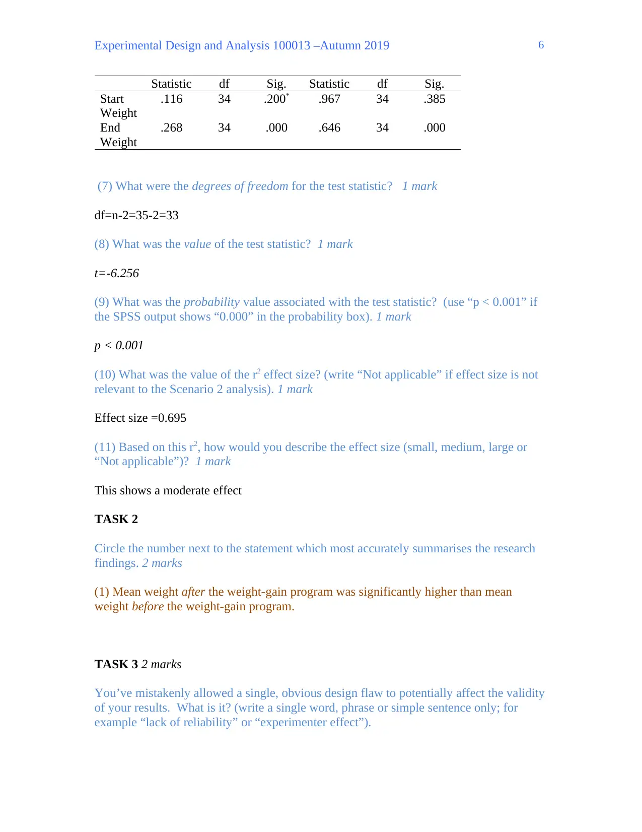
Statistic df Sig. Statistic df Sig.
Start
Weight
.116 34 .200* .967 34 .385
End
Weight
.268 34 .000 .646 34 .000
(7) What were the degrees of freedom for the test statistic? 1 mark
df=n-2=35-2=33
(8) What was the value of the test statistic? 1 mark
t=-6.256
(9) What was the probability value associated with the test statistic? (use “p < 0.001” if
the SPSS output shows “0.000” in the probability box). 1 mark
p < 0.001
(10) What was the value of the r2 effect size? (write “Not applicable” if effect size is not
relevant to the Scenario 2 analysis). 1 mark
Effect size =0.695
(11) Based on this r2, how would you describe the effect size (small, medium, large or
“Not applicable”)? 1 mark
This shows a moderate effect
TASK 2
Circle the number next to the statement which most accurately summarises the research
findings. 2 marks
(1) Mean weight after the weight-gain program was significantly higher than mean
weight before the weight-gain program.
TASK 3 2 marks
You’ve mistakenly allowed a single, obvious design flaw to potentially affect the validity
of your results. What is it? (write a single word, phrase or simple sentence only; for
example “lack of reliability” or “experimenter effect”).
6
Experimental Design and Analysis 100013 –Autumn 2019
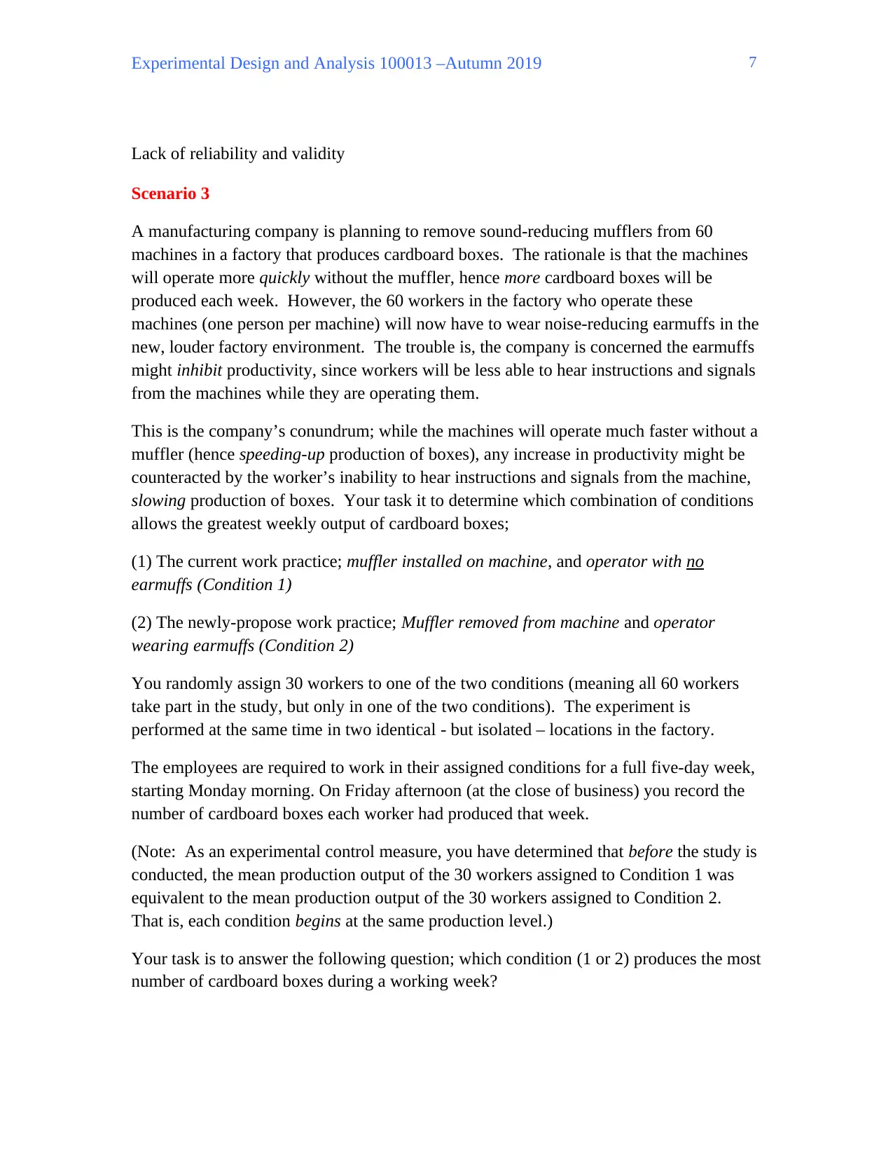
Lack of reliability and validity
Scenario 3
A manufacturing company is planning to remove sound-reducing mufflers from 60
machines in a factory that produces cardboard boxes. The rationale is that the machines
will operate more quickly without the muffler, hence more cardboard boxes will be
produced each week. However, the 60 workers in the factory who operate these
machines (one person per machine) will now have to wear noise-reducing earmuffs in the
new, louder factory environment. The trouble is, the company is concerned the earmuffs
might inhibit productivity, since workers will be less able to hear instructions and signals
from the machines while they are operating them.
This is the company’s conundrum; while the machines will operate much faster without a
muffler (hence speeding-up production of boxes), any increase in productivity might be
counteracted by the worker’s inability to hear instructions and signals from the machine,
slowing production of boxes. Your task it to determine which combination of conditions
allows the greatest weekly output of cardboard boxes;
(1) The current work practice; muffler installed on machine, and operator with no
earmuffs (Condition 1)
(2) The newly-propose work practice; Muffler removed from machine and operator
wearing earmuffs (Condition 2)
You randomly assign 30 workers to one of the two conditions (meaning all 60 workers
take part in the study, but only in one of the two conditions). The experiment is
performed at the same time in two identical - but isolated – locations in the factory.
The employees are required to work in their assigned conditions for a full five-day week,
starting Monday morning. On Friday afternoon (at the close of business) you record the
number of cardboard boxes each worker had produced that week.
(Note: As an experimental control measure, you have determined that before the study is
conducted, the mean production output of the 30 workers assigned to Condition 1 was
equivalent to the mean production output of the 30 workers assigned to Condition 2.
That is, each condition begins at the same production level.)
Your task is to answer the following question; which condition (1 or 2) produces the most
number of cardboard boxes during a working week?
7
Paraphrase This Document
Need a fresh take? Get an instant paraphrase of this document with our AI Paraphraser
Experimental Design and Analysis 100013 –Autumn 2019
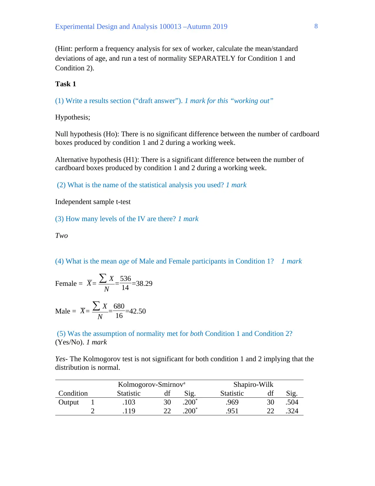
(Hint: perform a frequency analysis for sex of worker, calculate the mean/standard
deviations of age, and run a test of normality SEPARATELY for Condition 1 and
Condition 2).
Task 1
(1) Write a results section (“draft answer”). 1 mark for this “working out”
Hypothesis;
Null hypothesis (Ho): There is no significant difference between the number of cardboard
boxes produced by condition 1 and 2 during a working week.
Alternative hypothesis (H1): There is a significant difference between the number of
cardboard boxes produced by condition 1 and 2 during a working week.
(2) What is the name of the statistical analysis you used? 1 mark
Independent sample t-test
(3) How many levels of the IV are there? 1 mark
Two
(4) What is the mean age of Male and Female participants in Condition 1? 1 mark
Female = X = ∑ X
N = 536
14 =38.29
Male = X = ∑ X
N = 680
16 =42.50
(5) Was the assumption of normality met for both Condition 1 and Condition 2?
(Yes/No). 1 mark
Yes- The Kolmogorov test is not significant for both condition 1 and 2 implying that the
distribution is normal.
Condition
Kolmogorov-Smirnova Shapiro-Wilk
Statistic df Sig. Statistic df Sig.
Output 1 .103 30 .200* .969 30 .504
2 .119 22 .200* .951 22 .324
8
Experimental Design and Analysis 100013 –Autumn 2019
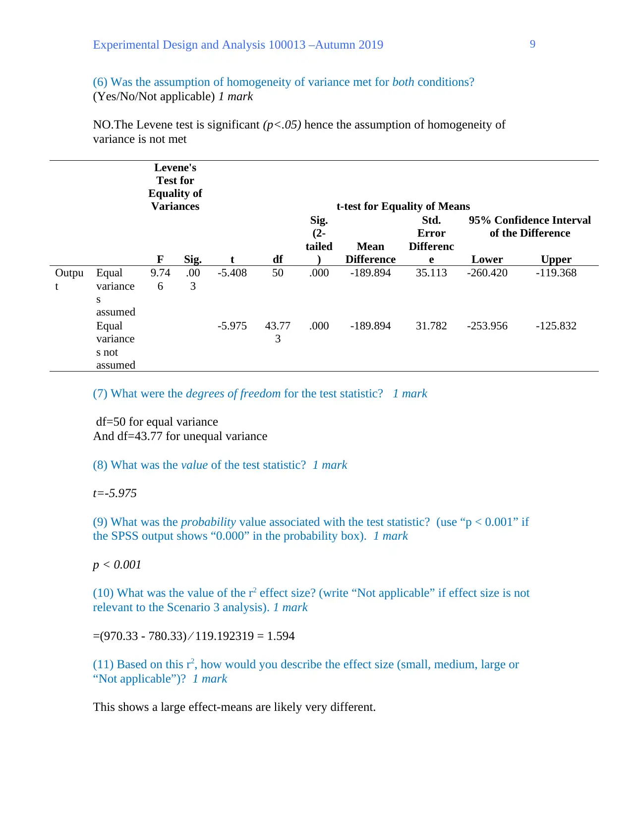
(6) Was the assumption of homogeneity of variance met for both conditions?
(Yes/No/Not applicable) 1 mark
NO.The Levene test is significant (p<.05) hence the assumption of homogeneity of
variance is not met
Levene's
Test for
Equality of
Variances t-test for Equality of Means
F Sig. t df
Sig.
(2-
tailed
)
Mean
Difference
Std.
Error
Differenc
e
95% Confidence Interval
of the Difference
Lower Upper
Outpu
t
Equal
variance
s
assumed
9.74
6
.00
3
-5.408 50 .000 -189.894 35.113 -260.420 -119.368
Equal
variance
s not
assumed
-5.975 43.77
3
.000 -189.894 31.782 -253.956 -125.832
(7) What were the degrees of freedom for the test statistic? 1 mark
df=50 for equal variance
And df=43.77 for unequal variance
(8) What was the value of the test statistic? 1 mark
t=-5.975
(9) What was the probability value associated with the test statistic? (use “p < 0.001” if
the SPSS output shows “0.000” in the probability box). 1 mark
p < 0.001
(10) What was the value of the r2 effect size? (write “Not applicable” if effect size is not
relevant to the Scenario 3 analysis). 1 mark
=(970.33 - 780.33) ⁄ 119.192319 = 1.594
(11) Based on this r2, how would you describe the effect size (small, medium, large or
“Not applicable”)? 1 mark
This shows a large effect-means are likely very different.
9
Experimental Design and Analysis 100013 –Autumn 2019
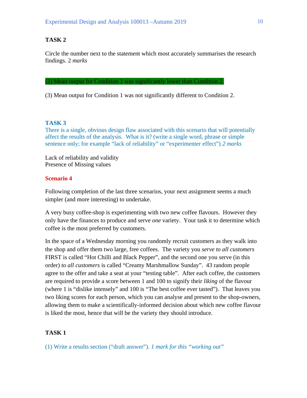
TASK 2
Circle the number next to the statement which most accurately summarises the research
findings. 2 marks
(2) Mean output for Condition 1 was significantly lower than Condition 2.
(3) Mean output for Condition 1 was not significantly different to Condition 2.
TASK 3
There is a single, obvious design flaw associated with this scenario that will potentially
affect the results of the analysis. What is it? (write a single word, phrase or simple
sentence only; for example “lack of reliability” or “experimenter effect”) 2 marks
Lack of reliability and validity
Presence of Missing values
Scenario 4
Following completion of the last three scenarios, your next assignment seems a much
simpler (and more interesting) to undertake.
A very busy coffee-shop is experimenting with two new coffee flavours. However they
only have the finances to produce and serve one variety. Your task it to determine which
coffee is the most preferred by customers.
In the space of a Wednesday morning you randomly recruit customers as they walk into
the shop and offer them two large, free coffees. The variety you serve to all customers
FIRST is called “Hot Chilli and Black Pepper”, and the second one you serve (in this
order) to all customers is called “Creamy Marshmallow Sunday”. 43 random people
agree to the offer and take a seat at your “testing table”. After each coffee, the customers
are required to provide a score between 1 and 100 to signify their liking of the flavour
(where 1 is “dislike intensely” and 100 is “The best coffee ever tasted”). That leaves you
two liking scores for each person, which you can analyse and present to the shop-owners,
allowing them to make a scientifically-informed decision about which new coffee flavour
is liked the most, hence that will be the variety they should introduce.
TASK 1
(1) Write a results section (“draft answer”). 1 mark for this “working out”
10
Secure Best Marks with AI Grader
Need help grading? Try our AI Grader for instant feedback on your assignments.
Experimental Design and Analysis 100013 –Autumn 2019
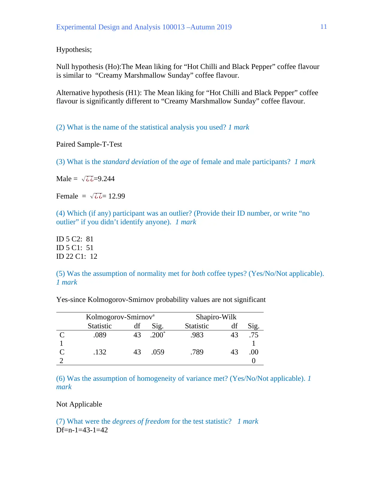
Hypothesis;
Null hypothesis (Ho):The Mean liking for “Hot Chilli and Black Pepper” coffee flavour
is similar to “Creamy Marshmallow Sunday” coffee flavour.
Alternative hypothesis (H1): The Mean liking for “Hot Chilli and Black Pepper” coffee
flavour is significantly different to “Creamy Marshmallow Sunday” coffee flavour.
(2) What is the name of the statistical analysis you used? 1 mark
Paired Sample-T-Test
(3) What is the standard deviation of the age of female and male participants? 1 mark
Male = √¿ ¿=9.244
Female = √¿ ¿= 12.99
(4) Which (if any) participant was an outlier? (Provide their ID number, or write “no
outlier” if you didn’t identify anyone). 1 mark
ID 5 C2: 81
ID 5 C1: 51
ID 22 C1: 12
(5) Was the assumption of normality met for both coffee types? (Yes/No/Not applicable).
1 mark
Yes-since Kolmogorov-Smirnov probability values are not significant
Kolmogorov-Smirnova Shapiro-Wilk
Statistic df Sig. Statistic df Sig.
C
1
.089 43 .200* .983 43 .75
1
C
2
.132 43 .059 .789 43 .00
0
(6) Was the assumption of homogeneity of variance met? (Yes/No/Not applicable). 1
mark
Not Applicable
(7) What were the degrees of freedom for the test statistic? 1 mark
Df=n-1=43-1=42
11
Experimental Design and Analysis 100013 –Autumn 2019
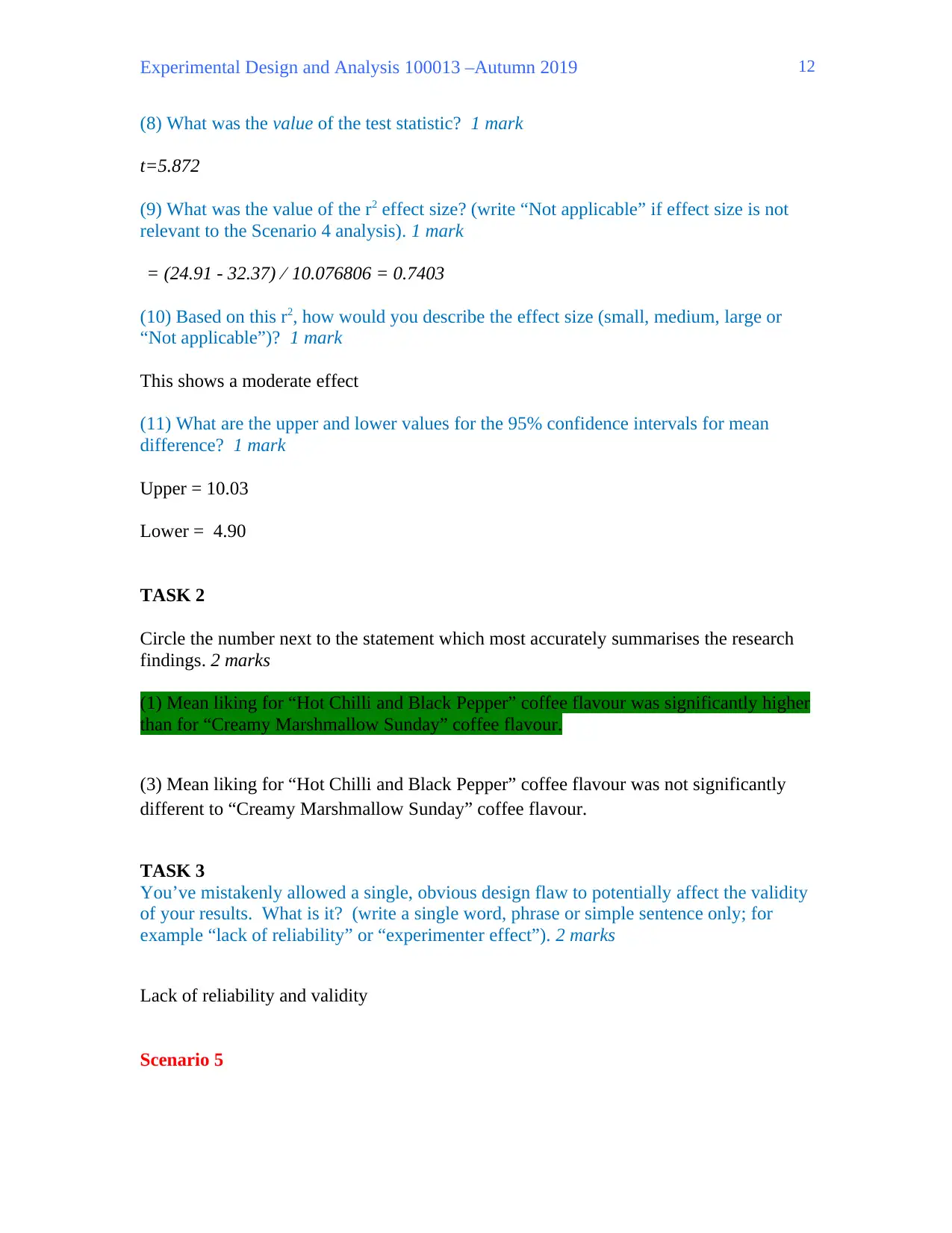
(8) What was the value of the test statistic? 1 mark
t=5.872
(9) What was the value of the r2 effect size? (write “Not applicable” if effect size is not
relevant to the Scenario 4 analysis). 1 mark
= (24.91 - 32.37) ⁄ 10.076806 = 0.7403
(10) Based on this r2, how would you describe the effect size (small, medium, large or
“Not applicable”)? 1 mark
This shows a moderate effect
(11) What are the upper and lower values for the 95% confidence intervals for mean
difference? 1 mark
Upper = 10.03
Lower = 4.90
TASK 2
Circle the number next to the statement which most accurately summarises the research
findings. 2 marks
(1) Mean liking for “Hot Chilli and Black Pepper” coffee flavour was significantly higher
than for “Creamy Marshmallow Sunday” coffee flavour.
(3) Mean liking for “Hot Chilli and Black Pepper” coffee flavour was not significantly
different to “Creamy Marshmallow Sunday” coffee flavour.
TASK 3
You’ve mistakenly allowed a single, obvious design flaw to potentially affect the validity
of your results. What is it? (write a single word, phrase or simple sentence only; for
example “lack of reliability” or “experimenter effect”). 2 marks
Lack of reliability and validity
Scenario 5
12
Experimental Design and Analysis 100013 –Autumn 2019
The IT (Information Technology) department of a very large accounting firm wants to
know whether their employees’ work satisfaction is stronger NOW than it was 10 years
ago. Specifically, department managers are hoping work satisfaction scores are higher
than they were in 2009, measured using the validated “Satisfaction at Work” scale (a
number from 1-100, where 1 is “extremely unhappy”, and 100 is “couldn’t be happier”).
Your task is to answer the firm’s question – are employees happier now in 2019 than in
2009? There were 38 employees in 2009, the (population) mean happiness score was 50
and the (population) standard deviation was 10 (the mean age of these employees was
also 82 years).
You administer the “Satisfaction at Work” scale to the current 40 employees (the
population) and compare their mean score with the 2009 employee group (no employee
in the current 40 was working for the company back in 2009). Can you give management
good news, that today’s employees are happier?
(Hint: the number 1.64 is important for this task – go to your lecture and tutorial notes to
track down why)
TASK 1
(1) Write a results section (“draft answer”). 1 mark for this “working out”
Hypothesis;
Null hypothesis (Ho): There is no difference in employees’ happiness levels between
2019 than in 2009
Alternative hypothesis (H1): employees are happier now in 2019 than in 2009
(2) What is the name of the statistical analysis you used? 1 mark
Sample t-test
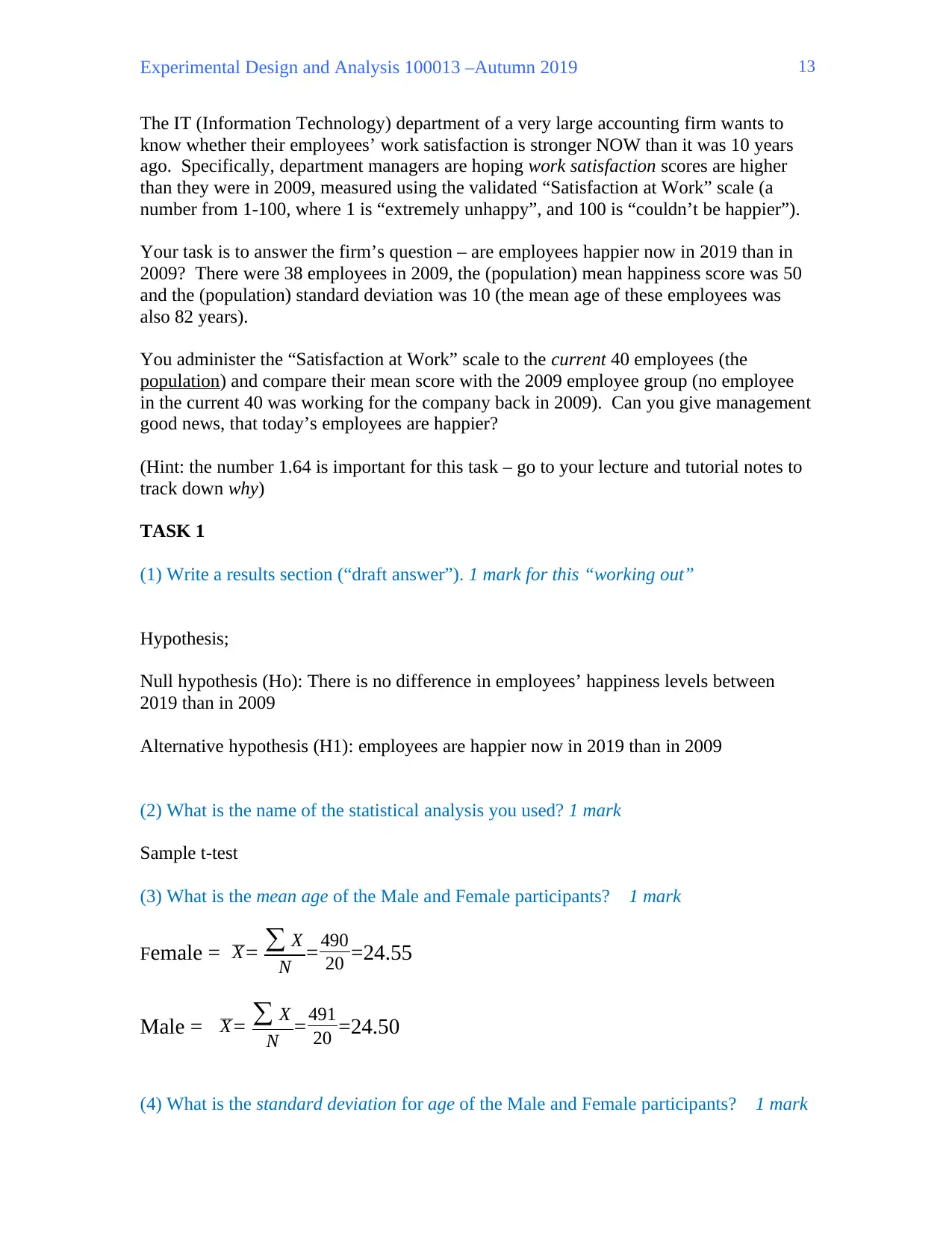
(3) What is the mean age of the Male and Female participants? 1 mark
Female = X = ∑ X
N =490
20 =24.55
Male = X = ∑ X
N = 491
20 =24.50
(4) What is the standard deviation for age of the Male and Female participants? 1 mark
13
The IT (Information Technology) department of a very large accounting firm wants to
know whether their employees’ work satisfaction is stronger NOW than it was 10 years
ago. Specifically, department managers are hoping work satisfaction scores are higher
than they were in 2009, measured using the validated “Satisfaction at Work” scale (a
number from 1-100, where 1 is “extremely unhappy”, and 100 is “couldn’t be happier”).
Your task is to answer the firm’s question – are employees happier now in 2019 than in
2009? There were 38 employees in 2009, the (population) mean happiness score was 50
and the (population) standard deviation was 10 (the mean age of these employees was
also 82 years).
You administer the “Satisfaction at Work” scale to the current 40 employees (the
population) and compare their mean score with the 2009 employee group (no employee
in the current 40 was working for the company back in 2009). Can you give management
good news, that today’s employees are happier?
(Hint: the number 1.64 is important for this task – go to your lecture and tutorial notes to
track down why)
TASK 1
(1) Write a results section (“draft answer”). 1 mark for this “working out”
Hypothesis;
Null hypothesis (Ho): There is no difference in employees’ happiness levels between
2019 than in 2009
Alternative hypothesis (H1): employees are happier now in 2019 than in 2009
(2) What is the name of the statistical analysis you used? 1 mark
Sample t-test
(3) What is the mean age of the Male and Female participants? 1 mark
Female = X = ∑ X
N =490
20 =24.55
Male = X = ∑ X
N = 491
20 =24.50
(4) What is the standard deviation for age of the Male and Female participants? 1 mark
13
Paraphrase This Document
Need a fresh take? Get an instant paraphrase of this document with our AI Paraphraser
Experimental Design and Analysis 100013 –Autumn 2019
Male = √¿ ¿=3.776
Female = √¿ ¿= 3.649
(5) Which (if any) participant was an outlier? (Provide their ID number, or write “no
outlier” if you didn’t identify anyone). 1 mark
NO Outlier
(6) If there was an outlier, what number did you change their score to? (write “Not
applicable” if there was no outlier). 1 mark
Not Applicable
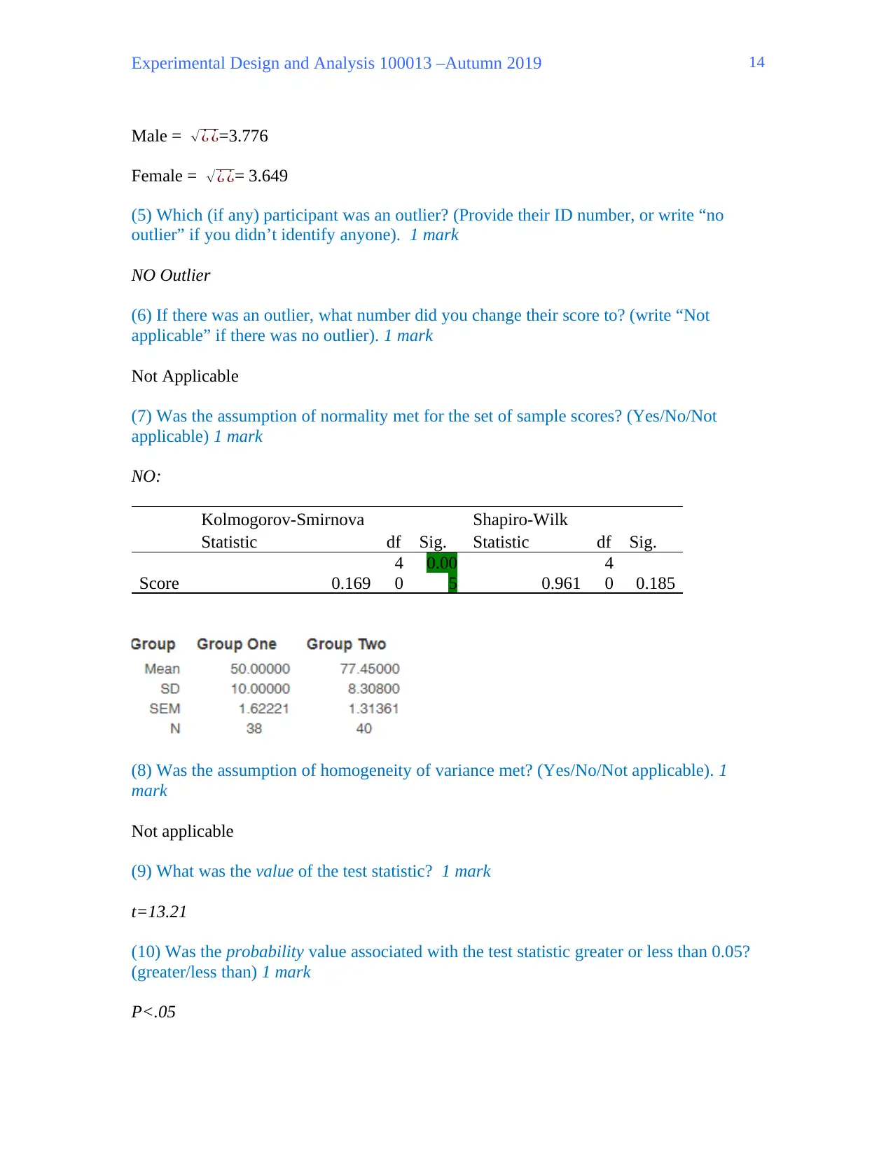
(7) Was the assumption of normality met for the set of sample scores? (Yes/No/Not
applicable) 1 mark
NO:
Kolmogorov-Smirnova Shapiro-Wilk
Statistic df Sig. Statistic df Sig.
Score 0.169
4
0
0.00
5 0.961
4
0 0.185
(8) Was the assumption of homogeneity of variance met? (Yes/No/Not applicable). 1
mark
Not applicable
(9) What was the value of the test statistic? 1 mark
t=13.21
(10) Was the probability value associated with the test statistic greater or less than 0.05?
(greater/less than) 1 mark
P<.05
14
Male = √¿ ¿=3.776
Female = √¿ ¿= 3.649
(5) Which (if any) participant was an outlier? (Provide their ID number, or write “no
outlier” if you didn’t identify anyone). 1 mark
NO Outlier
(6) If there was an outlier, what number did you change their score to? (write “Not
applicable” if there was no outlier). 1 mark
Not Applicable
(7) Was the assumption of normality met for the set of sample scores? (Yes/No/Not
applicable) 1 mark
NO:
Kolmogorov-Smirnova Shapiro-Wilk
Statistic df Sig. Statistic df Sig.
Score 0.169
4
0
0.00
5 0.961
4
0 0.185
(8) Was the assumption of homogeneity of variance met? (Yes/No/Not applicable). 1
mark
Not applicable
(9) What was the value of the test statistic? 1 mark
t=13.21
(10) Was the probability value associated with the test statistic greater or less than 0.05?
(greater/less than) 1 mark
P<.05
14
Experimental Design and Analysis 100013 –Autumn 2019
(11) In this style of statistical test, the value of 1.64 is important. What probability does
this correspond to? (Hint: provide a probability value here, rounded to two decimal
places). 1 mark
This is the computed value of t, which one compares with the tabulated value.
TASK 2
Circle the number next to the statement which most accurately summarises the research
findings. 2 marks
(1) Mean “work satisfaction” is significantly higher in 2019 employees compared to 2009
employees.
TASK 3
There is a single, obvious design flaw associated with this scenario that will potentially
affect the results of the analysis. What is it? (write a single word, phrase or simple
sentence only; for example “lack of reliability” or “experimenter effect”) 2 marks
Lack of reliability
Scenario 6
The same accounting firm is very happy with your work on the last project (Scenario 5).
Now they want to know if their proposed “Love your Job” campaign will improve
current employees’ work satisfaction in 2019. This applies to ALL employees, not just
the 40 in the IT department you utilised in Scenario 5.
Specifically, at the completion of the “Love your Job” campaign, will those employees
who were initially the least happy show an improved work satisfaction score that is now
equivalent to the happiest employees?
Before the firm implements their campaign, you administer a validated survey to measure
the “work satisfaction” of the 147 employees in the company. The survey measures
employee’s attitudes about their current employment status, and their future in the firm,
on a scale from 0-10; where a low score signifies low job satisfaction, and a high score
signifies high job satisfaction.
From the 147 scores, you select the bottom-scoring 25 employees (indicating very low
job satisfaction) and the top-scoring 25 employees (indicating very high job satisfaction).
The bottom-scoring employees provide a mean score of approximately 4 out of 10. The
top-scoring employees provide a mean score of approximately 9 out of 10.
15
Experimental Design and Analysis 100013 –Autumn 2019
The firm then implements the month-long “Love your Job” campaign (which involves
daily activities employees must complete with the expectation that they’ll love their job
more at the end of the month than they did at the beginning of the month).
At the conclusion of the month-long campaign you re-call the 50 employees (25 low
satisfaction, 25 high satisfaction) and ask them to complete a second, equivalent “work
satisfaction” survey which also uses a 0-10 scale, where the higher the score, the more
positive the participant’s work satisfaction. You assume that the campaign will not
necessarily improve scores for the high job satisfaction employees (since they’re as
happy as they can ever be). However, you expect scores will improve for the low job
satisfaction group.
Therefore, assuming the “Love your Work” campaign is valid and can improve employee
work satisfaction, you predict that the mean score of the low satisfaction group following
the campaign will increase and be equivalent to the mean score of the high satisfaction
group.
(Hint: perform a frequency analysis for sex of employee, calculate the mean/standard
deviations of age, and run a test of normality SEPARATELY for Condition 1 and
Condition 2).
TASK 1
(1) Write a results section (“draft answer”). 1 mark for this “working out”
Null hypothesis: There is no significant difference in Means for “work satisfaction” and
“low satisfaction” employee groups compared to the mean for the “high satisfaction”
employee group.
Alternative Hypothesis: The Mean “work satisfaction” is significantly higher for the “low
satisfaction” employee group compared to the mean for the “high satisfaction” employee
group.
(2) What is the name of the statistical analysis you used? 1 mark
Independent Sample T-Test
(3) What is the mean age of female and male participants in the high satisfaction group?
1 mark
Female = X = ∑ X
N =533
12 =44.42
16
Secure Best Marks with AI Grader
Need help grading? Try our AI Grader for instant feedback on your assignments.
Experimental Design and Analysis 100013 –Autumn 2019
Male = X = ∑ X
N = 568
13 =43.69
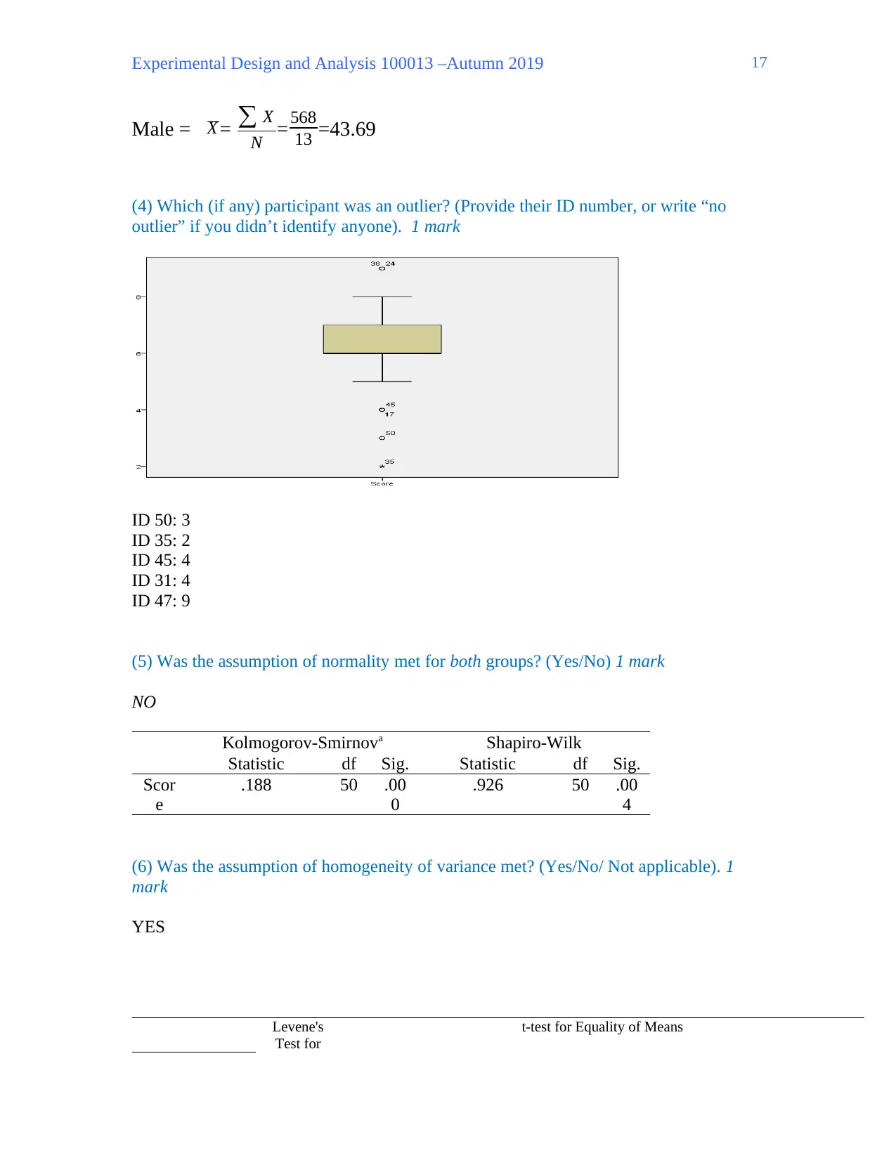
(4) Which (if any) participant was an outlier? (Provide their ID number, or write “no
outlier” if you didn’t identify anyone). 1 mark
ID 50: 3
ID 35: 2
ID 45: 4
ID 31: 4
ID 47: 9
(5) Was the assumption of normality met for both groups? (Yes/No) 1 mark
NO
Kolmogorov-Smirnova Shapiro-Wilk
Statistic df Sig. Statistic df Sig.
Scor
e
.188 50 .00
0
.926 50 .00
4
(6) Was the assumption of homogeneity of variance met? (Yes/No/ Not applicable). 1
mark
YES
Levene's
Test for
t-test for Equality of Means
17
Male = X = ∑ X
N = 568
13 =43.69
(4) Which (if any) participant was an outlier? (Provide their ID number, or write “no
outlier” if you didn’t identify anyone). 1 mark
ID 50: 3
ID 35: 2
ID 45: 4
ID 31: 4
ID 47: 9
(5) Was the assumption of normality met for both groups? (Yes/No) 1 mark
NO
Kolmogorov-Smirnova Shapiro-Wilk
Statistic df Sig. Statistic df Sig.
Scor
e
.188 50 .00
0
.926 50 .00
4
(6) Was the assumption of homogeneity of variance met? (Yes/No/ Not applicable). 1
mark
YES
Levene's
Test for
t-test for Equality of Means
17
Experimental Design and Analysis 100013 –Autumn 2019
Equality of
Variances
F Sig. t df
Sig. (2-
tailed)
Mean
Difference
Std. Error
Difference
95%
Confidence
Interval of the
Difference
Lower Upper
Score Equal
variances
assumed
.024 .879 .819 48 .417 .320 .391 -.466 1.106
Equal
variances
not
assumed
.819 47.996 .417 .320 .391 -.466 1.106
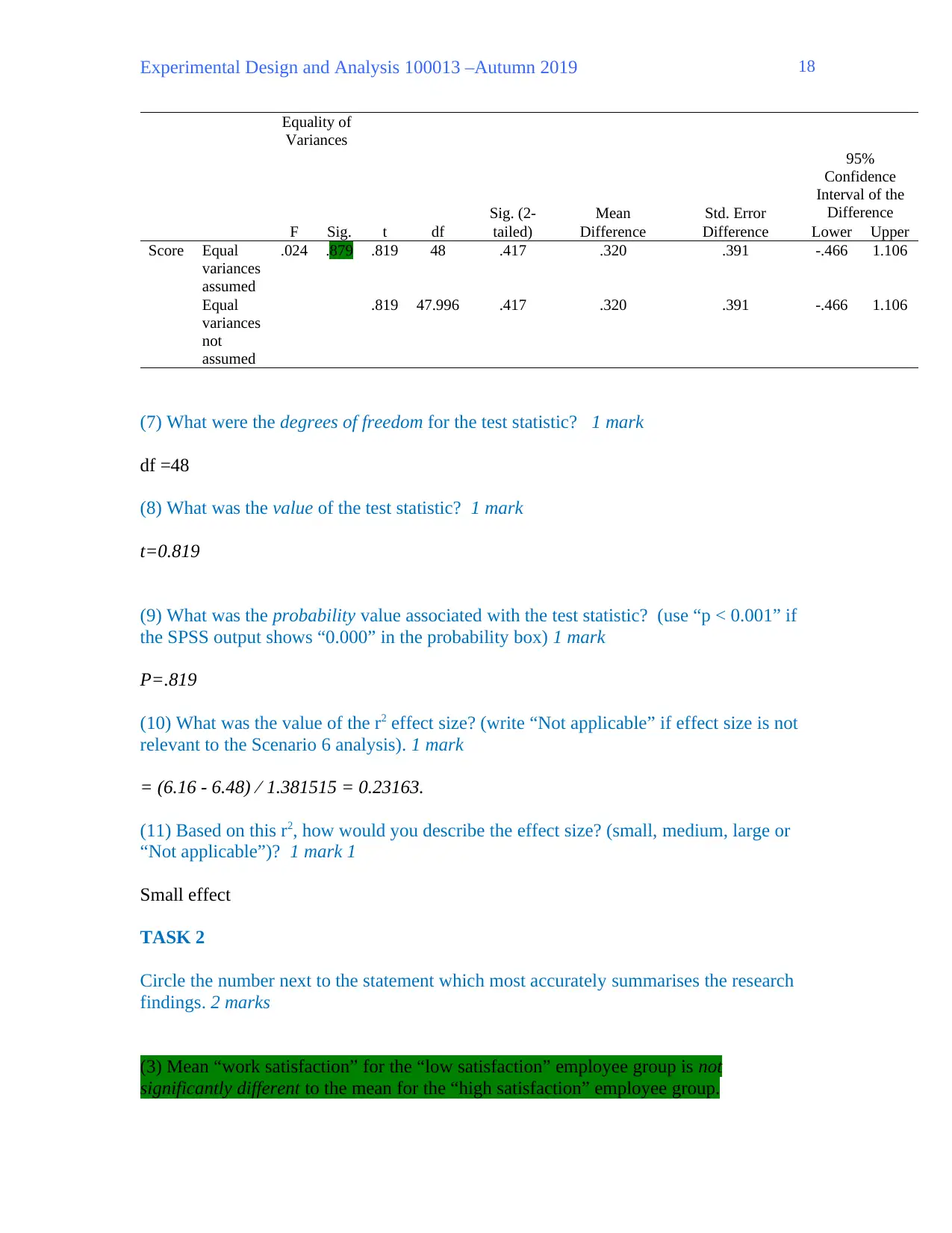
(7) What were the degrees of freedom for the test statistic? 1 mark
df =48
(8) What was the value of the test statistic? 1 mark
t=0.819
(9) What was the probability value associated with the test statistic? (use “p < 0.001” if
the SPSS output shows “0.000” in the probability box) 1 mark
P=.819
(10) What was the value of the r2 effect size? (write “Not applicable” if effect size is not
relevant to the Scenario 6 analysis). 1 mark
= (6.16 - 6.48) ⁄ 1.381515 = 0.23163.
(11) Based on this r2, how would you describe the effect size? (small, medium, large or
“Not applicable”)? 1 mark 1
Small effect
TASK 2
Circle the number next to the statement which most accurately summarises the research
findings. 2 marks
(3) Mean “work satisfaction” for the “low satisfaction” employee group is not
significantly different to the mean for the “high satisfaction” employee group.
18
Equality of
Variances
F Sig. t df
Sig. (2-
tailed)
Mean
Difference
Std. Error
Difference
95%
Confidence
Interval of the
Difference
Lower Upper
Score Equal
variances
assumed
.024 .879 .819 48 .417 .320 .391 -.466 1.106
Equal
variances
not
assumed
.819 47.996 .417 .320 .391 -.466 1.106
(7) What were the degrees of freedom for the test statistic? 1 mark
df =48
(8) What was the value of the test statistic? 1 mark
t=0.819
(9) What was the probability value associated with the test statistic? (use “p < 0.001” if
the SPSS output shows “0.000” in the probability box) 1 mark
P=.819
(10) What was the value of the r2 effect size? (write “Not applicable” if effect size is not
relevant to the Scenario 6 analysis). 1 mark
= (6.16 - 6.48) ⁄ 1.381515 = 0.23163.
(11) Based on this r2, how would you describe the effect size? (small, medium, large or
“Not applicable”)? 1 mark 1
Small effect
TASK 2
Circle the number next to the statement which most accurately summarises the research
findings. 2 marks
(3) Mean “work satisfaction” for the “low satisfaction” employee group is not
significantly different to the mean for the “high satisfaction” employee group.
18
Experimental Design and Analysis 100013 –Autumn 2019
TASK 3
You’ve mistakenly allowed a single, obvious design flaw to potentially affect the validity
of your results. What is it? (write a single word, phrase or simple sentence only; for
example “lack of reliability” or “experimenter effect”) 2 marks
Lack of reliability
END OF ASSESSMENT 1
19
TASK 3
You’ve mistakenly allowed a single, obvious design flaw to potentially affect the validity
of your results. What is it? (write a single word, phrase or simple sentence only; for
example “lack of reliability” or “experimenter effect”) 2 marks
Lack of reliability
END OF ASSESSMENT 1
19
1 out of 19
Related Documents


Your All-in-One AI-Powered Toolkit for Academic Success.
+13062052269
info@desklib.com
Available 24*7 on WhatsApp / Email
![[object Object]](/_next/static/media/star-bottom.7253800d.svg)
Unlock your academic potential
© 2024 | Zucol Services PVT LTD | All rights reserved.