Calculating t-tests for Independent and Paired Samples - Exercise 31 and 32

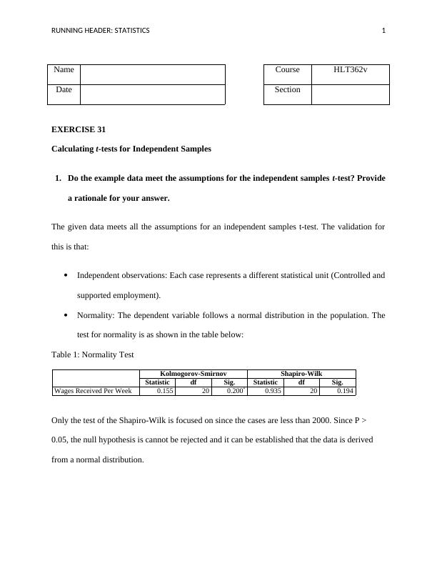
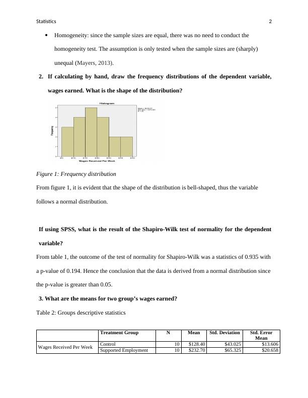
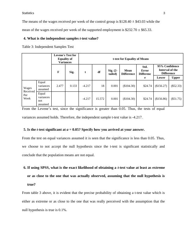
Exercise 31 and 32 of HLT362v course covers calculating t-tests for independent and paired samples. The exercises provide solved examples with assumptions, means, t-test values, and interpretations. The impact of supported employment vocational rehabilitation on wages earned and rehabilitation on emotional distress levels are also discussed. Weaknesses of the design are also highlighted.

RUNNING HEADER: STATISTICS 1
Name Course HLT362v
Date Section
EXERCISE 31
Calculating t-tests for Independent Samples
1. Do the example data meet the assumptions for the independent samples t-test? Provide
a rationale for your answer.
The given data meets all the assumptions for an independent samples t-test. The validation for
this is that:
 Independent observations: Each case represents a different statistical unit (Controlled and
supported employment).
 Normality: The dependent variable follows a normal distribution in the population. The
test for normality is as shown in the table below:
Table 1: Normality Test
Kolmogorov-Smirnov Shapiro-Wilk
Statistic df Sig. Statistic df Sig.
Wages Received Per Week 0.155 20 0.200* 0.935 20 0.194
Only the test of the Shapiro-Wilk is focused on since the cases are less than 2000. Since P >
0.05, the null hypothesis is cannot be rejected and it can be established that the data is derived
from a normal distribution.

Statistics 2
 Homogeneity: since the sample sizes are equal, there was no need to conduct the
homogeneity test. The assumption is only tested when the sample sizes are (sharply)
unequal (Mayers, 2013).
2. If calculating by hand, draw the frequency distributions of the dependent variable,
wages earned. What is the shape of the distribution?
Figure 1: Frequency distribution
From figure 1, it is evident that the shape of the distribution is bell-shaped, thus the variable
follows a normal distribution.
If using SPSS, what is the result of the Shapiro-Wilk test of normality for the dependent
variable?
From table 1, the outcome of the test of normality for Shapiro-Wilk was a statistics of 0.935 with
a p-value of 0.194. Hence the conclusion that the data is derived from a normal distribution since
the p-value is greater than 0.05.
3. What are the means for two group’s wages earned?
Table 2: Groups descriptive statistics
Treatment Group N Mean Std. Deviation Std. Error
Mean
Wages Received Per Week Control 10 $128.40 $43.025 $13.606
Supported Employment 10 $232.70 $65.325 $20.658

Statistics 3
The means of the wages received per week of the control group is $128.40 ± $43.03 while the
mean of the wages received per week of the supported employment is $232.70 ± $65.33.
4. What is the independent samples t-test value?
Table 3: Independent Samples Test
Levene's Test for
Equality of
Variances
t-test for Equality of Means
F Sig. t df Sig. (2-
tailed)
Mean
Difference
Std.
Error
Differenc
e
95% Confidence
Interval of the
Difference
Lower Upper
Wages
Received
Per
Week
Equal
variances
assumed
2.477 0.133 -4.217 18 0.001 ($104.30) $24.74 ($156.27) ($52.33)
Equal
variances
not
assumed
-4.217 15.572 0.001 ($104.30) $24.74 ($156.86) ($51.75)
From the Levene’s test, since the significance is greater than 0.05. Thus, the tests of equal
variances assumed holds. Therefore, the independent sample t-test value is -4.217.
5. Is the t-test significant at a = 0.05? Specify how you arrived at your answer.
From the test on equal variances assumed it is seen that the significance is less than 0.05. Thus,
we choose to not accept the null hypothesis since the t-test is significant statistically and
conclude that the population means are not equal.
6. If using SPSS, what is the exact likelihood of obtaining a t-test value at least as extreme
or as close to the one that was actually observed, assuming that the null hypothesis is
true?
From table 3 above, it is evident that the precise probability of obtaining a t-test value which is
either as extreme or as close to the one that was really perceived with the assumption that the
null hypothesis is true is 0.1%.

Statistics 4
7. Which group earned the most money post-treatment?
From table 3 above, the mean difference is -$104.30. Thus, the change between the control
group and the supported employment group is -$104.30. Therefore, it can be concluded that the
group which earned most money post-treatment is the supported employment group.
8. Write your interpretation of the results, as you would in an APA-formatted journal.
The independent sample t-test was conducted with an aim to compare wage payment between
supported employment group and control group. There was a significant difference in the
averages for the control group (M=$128.4, SD=$43.03) and the supported employment group
(M=$232.7, SD=$65.33); t(18)=-4.2, p=0.001.
9. What do the results indicate regarding the impact of the supported employment
vocational rehabilitation on wages earned?
The outcomes suggest that the type of employment has an effect on the amount of wages one
receives. Thus, the supported employment vocational rehabilitation impacts the wages earned by
disabled veterans positively. The program can, therefore, be deemed to be beneficial.
10. Was the sample size adequate to detect significant differences between the two groups
in this example? Provide a rationale for your answer.
The sample size can be stated to be adequate in detecting the difference that is significant
between the two groups. The rationale of this argument can be supported by the results showing
the contrast between the average of the earned money, the t value, the p-value, and the groups’
confidence interval.

Statistics 5
EXERCISE 32
Calculating t-tests for Paired (Dependent) Samples
1. Do the data meet the assumptions for the paired samples t-test? Provide a rationale for
your answer.
It is evident that the data meet the assumptions for the paired samples t-test. The justification for
this argument is that the dependent variables are continuous (Ross & Willson, 2017).
Consequently, the dependent variables are independent of one another and also do not contain
any outliers.
2. If calculating by hand, draw the frequency distributions of the two variables. What are
the shapes of the distributions?
Figure 2: MPI Affective Distress Baseline Figure 3: MPI Affective Distress Post Tx
Based on figure 2 and 3 above, it is evident that the shapes of the distributions are bell-shaped.
Therefore, the two variables follow a normal distribution.
If using SPSS, what are the results of the Shapiro-Wilk tests of normality for the two
variables?
Table 4: Tests of Normality

Statistics 6
Kolmogorov-Smirnova Shapiro-Wilk
Statistic df Sig. Statistic df Sig.
MPI Affective Distress
Baseline
.134 10 .200* .953 10 .705
MPI Affective Distress Post Tx .235 10 .124 .912 10 .292
From table 4 above, the outcomes of the Shapiro-Wilk test of normality was a statistics of 0.953
with a p-value of 0.705 for MPI Affective Distress Baseline and a statistics of 0.912 with a p-
value equal to 0.292 for MPI Affective Distress Post Tx. Hence the conclusion that the two
variables have data coming from a normal distribution since the p-values are greater than 0.05.
3. What are the means for the baseline and post-treatment affective distress scores,
respectively?
Table 5: Paired Samples Statistics
Mean N Std. Deviation Std. Error Mean
Pair 1
MPI Affective Distress
Baseline
3.030 10 1.6640 .5262
MPI Affective Distress Post Tx 2.040 10 .9834 .3110
The average of the MPI Affective Distress Baseline is 3.03 ± 1.66 while the average of the MPI
Affective Distress Post Tx is 2.04 ± 0.98.
4. What is the paired samples t-test value?
Table 6: Paired Samples Test
Paired Differences
t df
Sig. (2-
tailed)Mean
Std.
Deviation
Std.
Error
Mean
95% Confidence
Interval of the
Difference
Lower Upper

Statistics 7
Pair 1 MPI
Affective
Distress
Baseline -
MPI
Affective
Distress
Post Tx
0.99 1.0929 0.3456 0.2082 1.7718 2.865 9 0.019
The paired sample t-test value as seen in table 6 is 2.865.
5. Is the t-test significant at α = 0.05? Specify how you arrived at your answer.
From table 6 above, the significance is 0.019. Since the p-value is less than 0.019, we choose to
accept the null hypothesis. Thus, the t-test is significant at the alpha level where it is equal to
0.05.
6. If using SPSS, what is the exact likelihood of obtaining a t-test value at least as extreme
as or as close to the one that was actually observed, assuming that the null hypothesis is
true?
Based on table 6, the exact probability of attaining a t-test value which is at least as extreme as or
as close to the one that was actually observed with an assumption that the null hypothesis is true
is 1.9%.
7. On average, did the affective distress scores improve or deteriorate over time? Provide
a rationale for your answer.
Evidently, the distress scores deteriorated over time. On average, the MPI Affective Distress
Baseline was higher than the MPI Affective Distress Post TX (95% CI [0.21, 1.77]) as seen by
the mean difference of 0.99.
8. Write your interpretation of the results as you would in an APA-formatted journal.

Statistics 8
The paired samples t-test was carried out so as to relate the different distress scores before
rehabilitation on emotional distress. There was a difference that was significant in the MPI
Affective Distress Baseline (M=3.03, SD=1.66) and MPI Affective Distress Post Tx (M=2.04,
SD=0.983); t(2.865)=, p=0.019.
9. What do the results indicate regarding the impact of the rehabilitation on emotional
distress levels?
The outcomes, therefore, suggest that the rehabilitation of emotional distress impacts positively
on the stress levels of an individual.
10. What are the weaknesses of the design in this example?
The study design involves the use of a low sample size. Thus, the derived results cannot be
generalized without using caution.

Statistics 9
Reference:
Mayers, A. (2013). Introduction to Statistics and SPSS in Psychology. Pearson Higher Ed.
Ross, A., & Willson, V. L. (2017). Paired Samples T-Test. In Basic and Advanced Statistical
Tests (pp. 17-19). SensePublishers, Rotterdam.