Machine Learning and Game Mechanics Analysis

The assignment delves into the concept of loss functions in machine learning, demonstrating their application in a game mechanics context. It outlines steps for deriving a combined loss function from initial equations and provides a detailed analysis of damage per second (DPS) calculations for a game drill attack. The analysis considers multiple attacks, recharge times, and calculates the DPS for each scenario.

Running head: ALGORITHM DESIGN WITH LOSS FUNCTIONS 1
Student Name
Institutional Affiliations
Course
Date

ALGORITHM DESIGN WITH LOSS FUNCTIONS 2
Problem 1: Multivariate Adaptive Regression Splines (MARS)
a). MARS can only be changed by employing of various binary search algorithm that
maintains the order of divide and conquer technique. One needs not settle on one method but
keeps giving it a try for a number of them as shown. Important is that the change of
procedure for MARS into a decision tree employees use of algorithmic design chosen at
random and only selection of method either through carrying recursion or iteration ( Becker,
2017). One of advantage of decision tree against MARS is that it allows one to use data in its
normal state. The decision tree are also not complicate like MARS and therefore they are easily
understood. In the interaction in decision tree it is easy to add odd variables unlike in Mars. You
also deal with minimal assumptions in decision tree.
It should also be noted that there are disadvantages of decision tree which arise due to its
inability to perform well. Trees are not perfect like Mars which is a disadvantage that puts
MARS ahead of trees. Trees require relatively large sample which can result to higher error
Let the x→ the house for such
Search(C, x, y) first ← C[i] middle ← C[(x + y)/2] last ← C[y]
if x ∈ {last,middle, first, }:
then
return loop for index
else :
if (x < last and x > first ) or (x > last and x > middle): [x for x > last ]
then
return SEARCH(C,(i + j)/2, x, y) else : return SEARCH(C, i,(x + y)/2, x)
The binary search tree for (C, i, j, x) employs recursion in the process for search. Failure to
search for the item, leads to debugging.
We first let k ≥ 0 for the number of points through which A was taken through. The proof
then is found when we try to trace k. It is achieved via binary search C[1 . . . z] and the “left
side” C[j + 1 . . . z].It is determined from the search that elements on the right are less than those
on the left
C[1] for j > 1 such that C[j] is larger than C[1]. It is thus in that k = j − 1
The upper bound for the search algorithm is chosen universally. It is because we can sort the
sequence in the form Log (N) for N unless it is the worst case scenario. It will thus need us to
gather permutation in the running time O log (N)
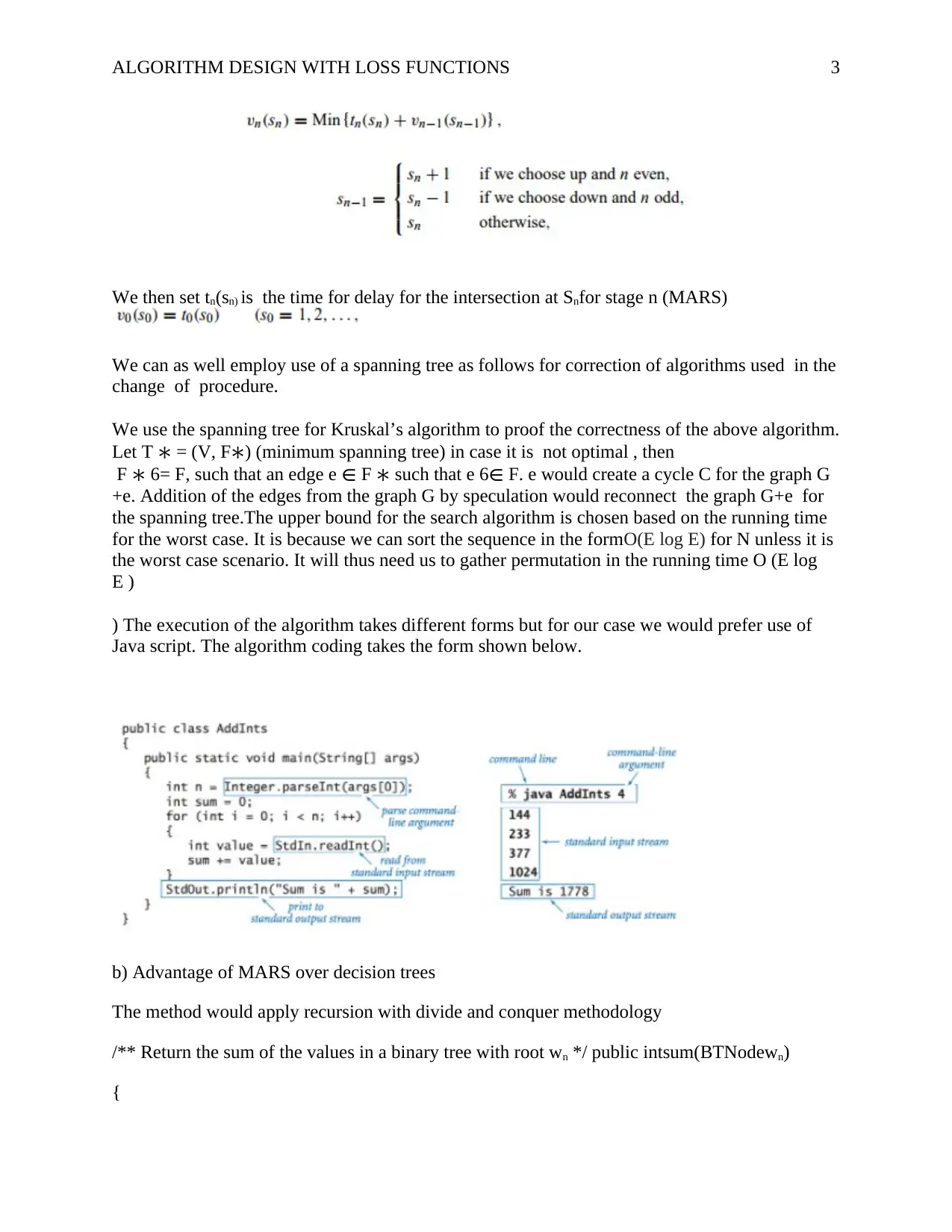
Begin by numbering the houses, say Sn=1 for bottom up to Sn= N for the upper intersection
subject to

ALGORITHM DESIGN WITH LOSS FUNCTIONS 3
We then set tn(sn) is the time for delay for the intersection at Snfor stage n (MARS)
We can as well employ use of a spanning tree as follows for correction of algorithms used in the
change of procedure.
We use the spanning tree for Kruskal’s algorithm to proof the correctness of the above algorithm.
Let T ∗ = (V, F∗) (minimum spanning tree) in case it is not optimal , then
F ∗ 6= F, such that an edge e ∈ F ∗ such that e 6∈ F. e would create a cycle C for the graph G
+e. Addition of the edges from the graph G by speculation would reconnect the graph G+e for
the spanning tree.The upper bound for the search algorithm is chosen based on the running time
for the worst case. It is because we can sort the sequence in the formO(E log E) for N unless it is
the worst case scenario. It will thus need us to gather permutation in the running time O (E log
E )
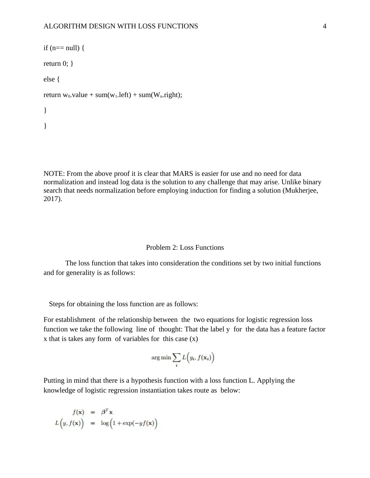
) The execution of the algorithm takes different forms but for our case we would prefer use of
Java script. The algorithm coding takes the form shown below.
b) Advantage of MARS over decision trees
The method would apply recursion with divide and conquer methodology
/** Return the sum of the values in a binary tree with root wn */ public intsum(BTNodewn)
{

ALGORITHM DESIGN WITH LOSS FUNCTIONS 4
if (n== null) {
return 0; }
else {
return w0.value + sum(w1.left) + sum(Wn.right);
}
}
NOTE: From the above proof it is clear that MARS is easier for use and no need for data
normalization and instead log data is the solution to any challenge that may arise. Unlike binary
search that needs normalization before employing induction for finding a solution (Mukherjee,
2017).
Problem 2: Loss Functions
The loss function that takes into consideration the conditions set by two initial functions
and for generality is as follows:
Steps for obtaining the loss function are as follows:
For establishment of the relationship between the two equations for logistic regression loss
function we take the following line of thought: That the label y for the data has a feature factor
x that is takes any form of variables for this case (x)
Putting in mind that there is a hypothesis function with a loss function L. Applying the
knowledge of logistic regression instantiation takes route as below:

ALGORITHM DESIGN WITH LOSS FUNCTIONS 5
And finally through application of natural logs integration by parts with limits chosen as ( 0,∞)
We get the real combination of the loss function as required;
By use of the attack character, we apply the 65.5 damage every second. The damage is assumed
for indefinite barring restrictions for the game (Ruela&Guimarães, 2017). Our case is the
drilling target. A single attack does not produce enough DPS to help take down the foe. It is thus
necessary for us to calculate a series for(Tessler et al,2017).
Damage per Second =Damage / (Activation Time + Recharge)
DPS = steel / IDDC
=65.5/2,5
=26.5 DPS
It means that original attack for the drill has approximately 26.5damage per second for
each activation drill. The time one of the drillers activates the second attack, the first one would
have recharged (Tessler et al,2017).For the second subsequent attack, it should be realized that is
way slower than the earlier one. Addition of a second attack t the earlier one results to a less slow
attack that may be 100 DAT. The DAT for this case takes 0.50sec, with a recharge of .75
seconds.

ALGORITHM DESIGN WITH LOSS FUNCTIONS 6
References
Becker, K. (2017). Software Deployment Analysis for Mixed Reliability Automotive
Systems (Doctoral dissertation, TechnischeUniversitätMünchen).
Mukherjee, A. (2017). Retrieval of Multimedia Information Using Content-Based Image
Retrieval (CBIR) Techniques. Intelligent Analysis of Multimedia Information, 143-180.
Ruela, A. S., &Guimarães, F. G. (2017).Procedural generation of non-player characters in
massively multiplayer online strategy games. Soft Computing, 21(23), 7005-7020.
Tessler, C., Givony, S., Zahavy, T., Mankowitz, D. J., &Mannor, S. (2017). A Deep Hierarchical
Approach to Lifelong Learning in Minecraft.In AAAI (pp. 1553-1561).