ICT110 Fatalities Analysis Report Australia - Sunshine Coast Uni 2019
VerifiedAdded on 2023/03/29
|12
|1650
|53
Report
AI Summary
This report presents an analysis of fatality trends in Australia between 2010 and 2018, focusing on state and gender-based comparisons. The study utilizes data from the World Bank and employs various statistical techniques including univariate and bivariate analysis, cluster analysis, and linear regression. Key findings indicate significant differences in fatality rates across different states and between genders, with female victims exhibiting a tendency for higher speed limits. The analysis also explores the relationship between speed limits and factors like Christmas periods. The report concludes by reflecting on the application of statistical techniques in deriving meaningful insights from the dataset and their importance in decision-making.
Analysis of fatalities in Australia
Prepared by
Firstname Lastname
University of the Sunshine Coast
Queensland
May-June 2019
Prepared by
Firstname Lastname
University of the Sunshine Coast
Queensland
May-June 2019
Paraphrase This Document
Need a fresh take? Get an instant paraphrase of this document with our AI Paraphraser
1. Introduction
1.1 Authorization and Purpose
This study sought to analyze the trends in fatalities in Australia. The aim was to
analyze and compare the trends based on the states as well as the gender. The
question that this study seeks to answer is how does the trend in fatalities compare for
the males and states? The findings of this study are crucial in informing the
government as well as other stakeholders on how to come up with measures that
would see the reduction in the fatalities.
1.2 Limitations
The main limitation of this study is the fact that the collected data is only for one
country which is Australia. There is therefore no comparison that is being made to
understand the trends in other countries.
1.3 Scope
Secondary data collected from the World bank database is utilized for this study.
Before analysis is done the dataset is pre-processed ready for analysis. Both
univariate and bivariate analysis are performed for this study. Other advanced
analysis involving regression analysis as well as cluster analysis are also performed.
1.4 Methodology
The study involves analysis of panel data. The data spans from 2010 through to 2018
and involving six states in Australia as well as two territories.
2. Data setup
The pre-processed data was loaded into R for analysis. The code used to load the data
into R is given below;
The necessary packages such as cluster package
were loaded into R. The code is presented below;
3. Exploratory Data analysis
3.1 One variable analysis
3.1.1 One variable analysis 1
The codes are presented below;
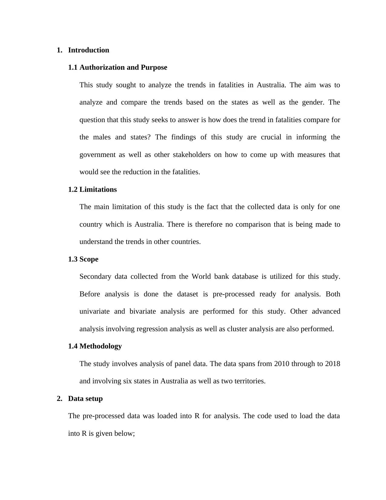
In this section, we present the summary statistics for Age. As
can be seen, the average age of the victims was found to be 43.77 with a median age being 41.00.
Since the median and the mean age are close to each other we can say that the distribution is
close to normal distribution. This is confirmed form the boxplot given below;
Figure 1: Box plot of speed limit
fatalities<-read.csv("C:\\
Users\\Documents\\
fatalities.csv")
install.packages("cluster")
library(cluster)
summary(fatalities$Age)
boxplot(fatalities$Age,
ylab="Age",
main="Boxplot of age",
col=" chartreuse1 ")
were loaded into R. The code is presented below;
3. Exploratory Data analysis
3.1 One variable analysis
3.1.1 One variable analysis 1
The codes are presented below;
In this section, we present the summary statistics for Age. As
can be seen, the average age of the victims was found to be 43.77 with a median age being 41.00.
Since the median and the mean age are close to each other we can say that the distribution is
close to normal distribution. This is confirmed form the boxplot given below;
Figure 1: Box plot of speed limit
fatalities<-read.csv("C:\\
Users\\Documents\\
fatalities.csv")
install.packages("cluster")
library(cluster)
summary(fatalities$Age)
boxplot(fatalities$Age,
ylab="Age",
main="Boxplot of age",
col=" chartreuse1 ")
⊘ This is a preview!⊘
Do you want full access?
Subscribe today to unlock all pages.
Trusted by 1+ million students worldwide
3.1.2 One variable analysis 2
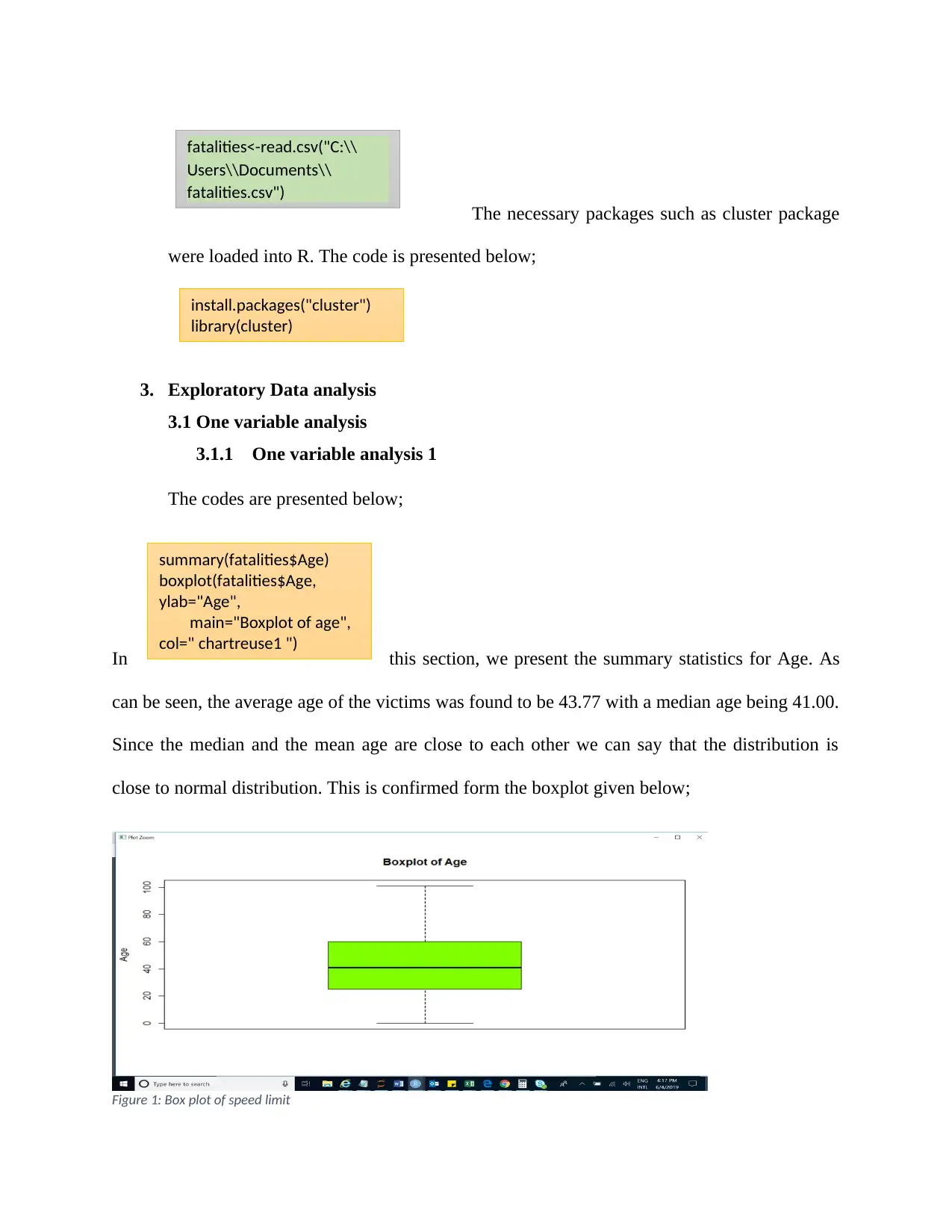
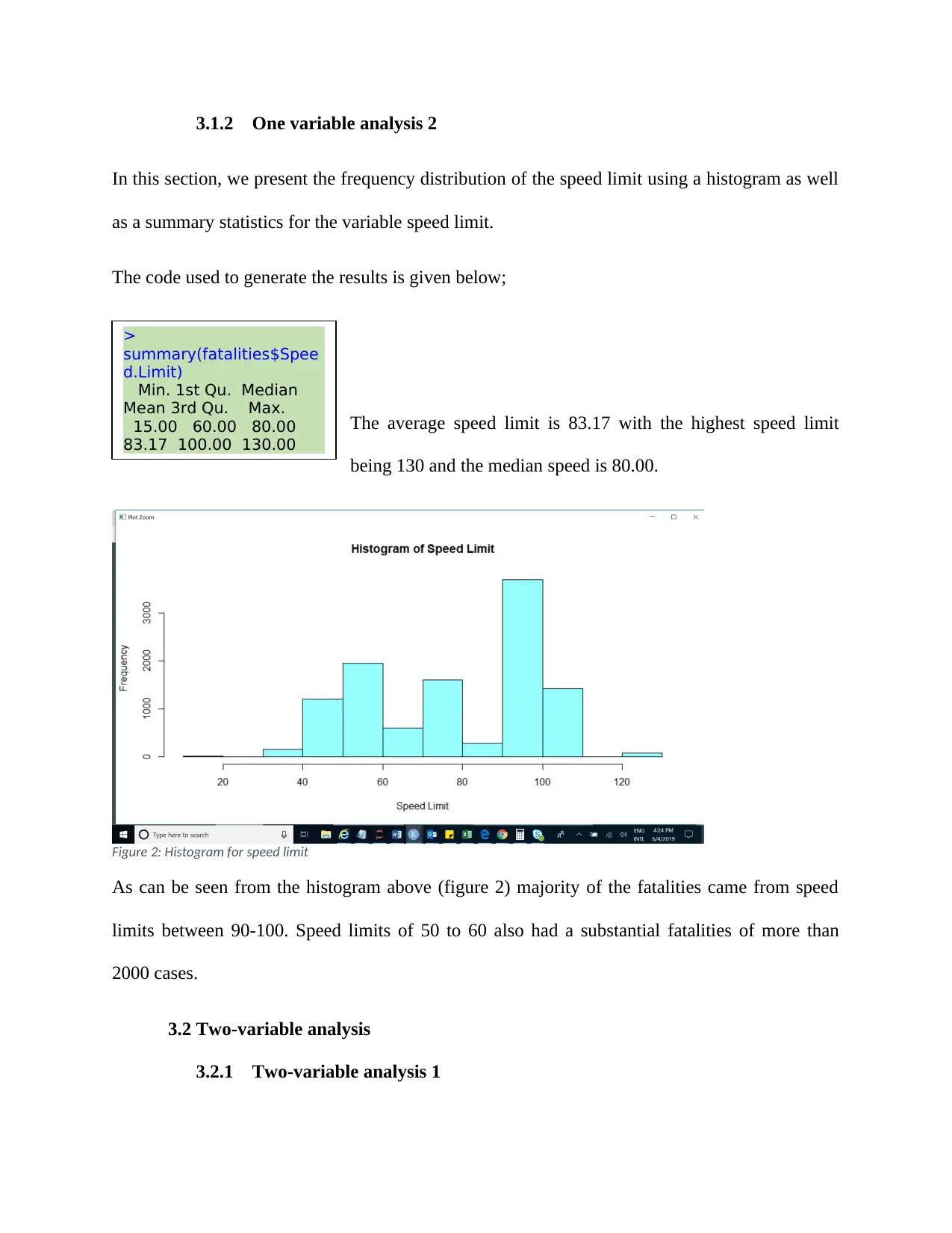
In this section, we present the frequency distribution of the speed limit using a histogram as well
as a summary statistics for the variable speed limit.
The code used to generate the results is given below;
The average speed limit is 83.17 with the highest speed limit
being 130 and the median speed is 80.00.
Figure 2: Histogram for speed limit
As can be seen from the histogram above (figure 2) majority of the fatalities came from speed
limits between 90-100. Speed limits of 50 to 60 also had a substantial fatalities of more than
2000 cases.
3.2 Two-variable analysis
3.2.1 Two-variable analysis 1
>
summary(fatalities$Spee
d.Limit)
Min. 1st Qu. Median
Mean 3rd Qu. Max.
15.00 60.00 80.00
83.17 100.00 130.00
Paraphrase This Document
Need a fresh take? Get an instant paraphrase of this document with our AI Paraphraser
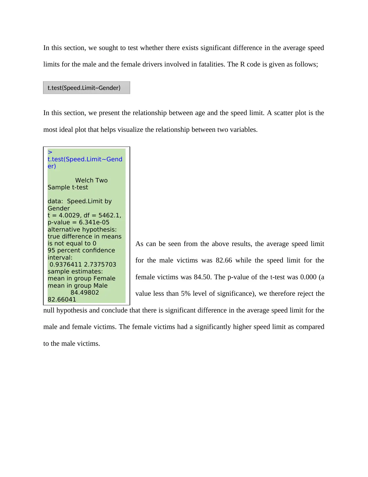
In this section, we sought to test whether there exists significant difference in the average speed
limits for the male and the female drivers involved in fatalities. The R code is given as follows;
In this section, we present the relationship between age and the speed limit. A scatter plot is the
most ideal plot that helps visualize the relationship between two variables.
As can be seen from the above results, the average speed limit
for the male victims was 82.66 while the speed limit for the
female victims was 84.50. The p-value of the t-test was 0.000 (a
value less than 5% level of significance), we therefore reject the
null hypothesis and conclude that there is significant difference in the average speed limit for the
male and female victims. The female victims had a significantly higher speed limit as compared
to the male victims.
t.test(Speed.Limit~Gender)
>
t.test(Speed.Limit~Gend
er)
Welch Two
Sample t-test
data: Speed.Limit by
Gender
t = 4.0029, df = 5462.1,
p-value = 6.341e-05
alternative hypothesis:
true difference in means
is not equal to 0
95 percent confidence
interval:
0.9376411 2.7375703
sample estimates:
mean in group Female
mean in group Male
84.49802
82.66041
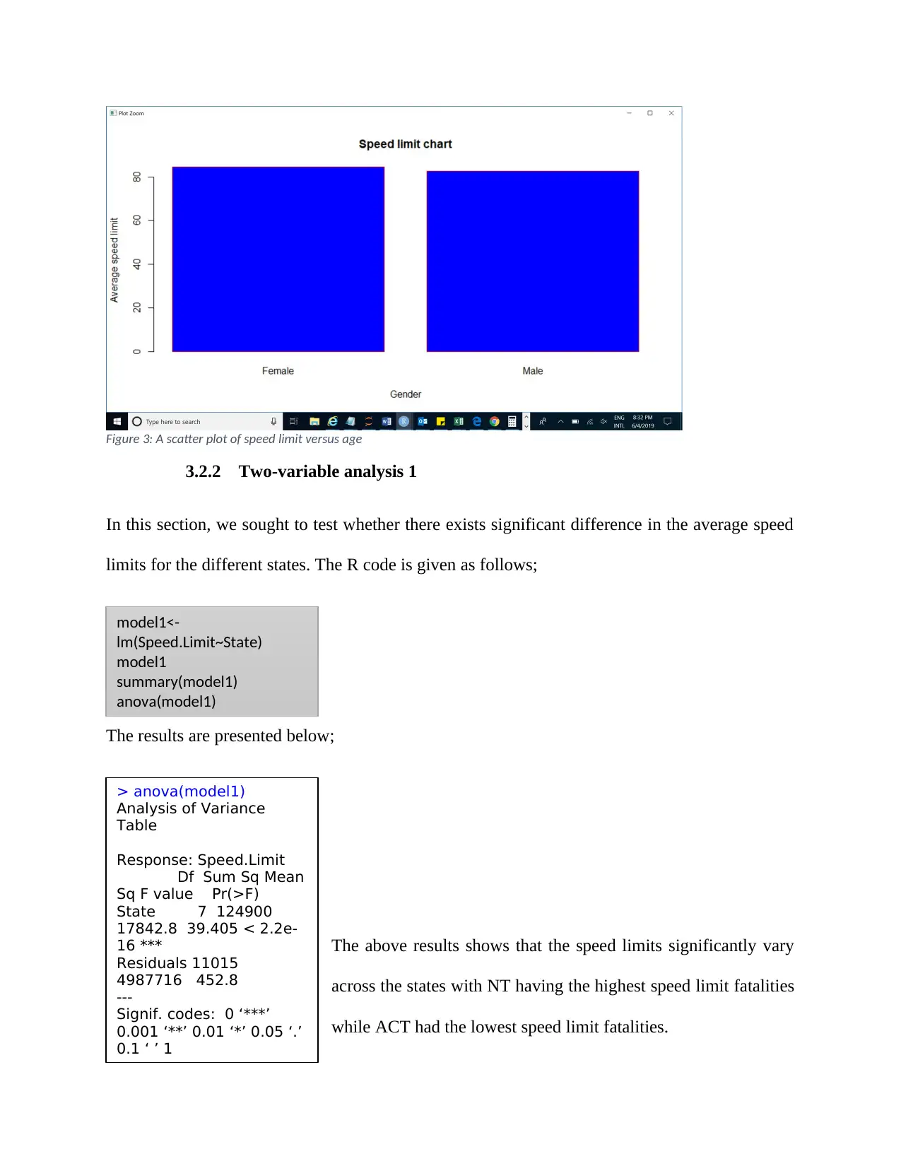
Figure 3: A scatter plot of speed limit versus age
3.2.2 Two-variable analysis 1
In this section, we sought to test whether there exists significant difference in the average speed
limits for the different states. The R code is given as follows;
The results are presented below;
The above results shows that the speed limits significantly vary
across the states with NT having the highest speed limit fatalities
while ACT had the lowest speed limit fatalities.
model1<-
lm(Speed.Limit~State)
model1
summary(model1)
anova(model1)
> anova(model1)
Analysis of Variance
Table
Response: Speed.Limit
Df Sum Sq Mean
Sq F value Pr(>F)
State 7 124900
17842.8 39.405 < 2.2e-
16 ***
Residuals 11015
4987716 452.8
---
Signif. codes: 0 ‘***’
0.001 ‘**’ 0.01 ‘*’ 0.05 ‘.’
0.1 ‘ ’ 1
⊘ This is a preview!⊘
Do you want full access?
Subscribe today to unlock all pages.
Trusted by 1+ million students worldwide
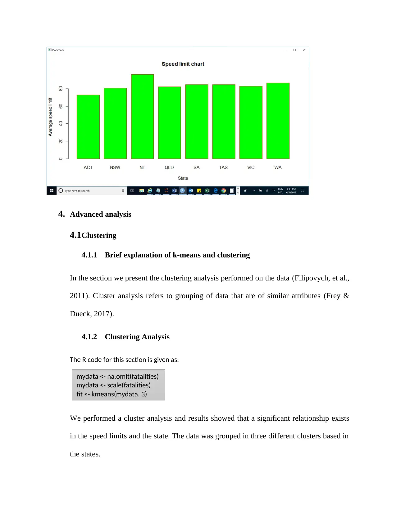
4. Advanced analysis
4.1Clustering
4.1.1 Brief explanation of k-means and clustering
In the section we present the clustering analysis performed on the data (Filipovych, et al.,
2011). Cluster analysis refers to grouping of data that are of similar attributes (Frey &
Dueck, 2017).
4.1.2 Clustering Analysis
The R code for this section is given as;
We performed a cluster analysis and results showed that a significant relationship exists
in the speed limits and the state. The data was grouped in three different clusters based in
the states.
mydata <- na.omit(fatalities)
mydata <- scale(fatalities)
fit <- kmeans(mydata, 3)
Paraphrase This Document
Need a fresh take? Get an instant paraphrase of this document with our AI Paraphraser
4.2 Linear regression
4.2.1 Brief definition of linear regression
In this section, we present regression analysis for predicting the speed limit (Aldrich,
2015). Regression analysis is a technique that tries to show a relationship that exists
between a dependent variable and one or more independent (exploratory) variables
(Tofallis, 2009). The simple linear regression equation is of the form;
Y = β0 +β1 X
Where Y is the dependent (response) variable, β0 is the intercept coefficient, β1 is the
coefficient of X and last X is the independent (exploratory) variable (Mahdavi
Damghani, 2012).
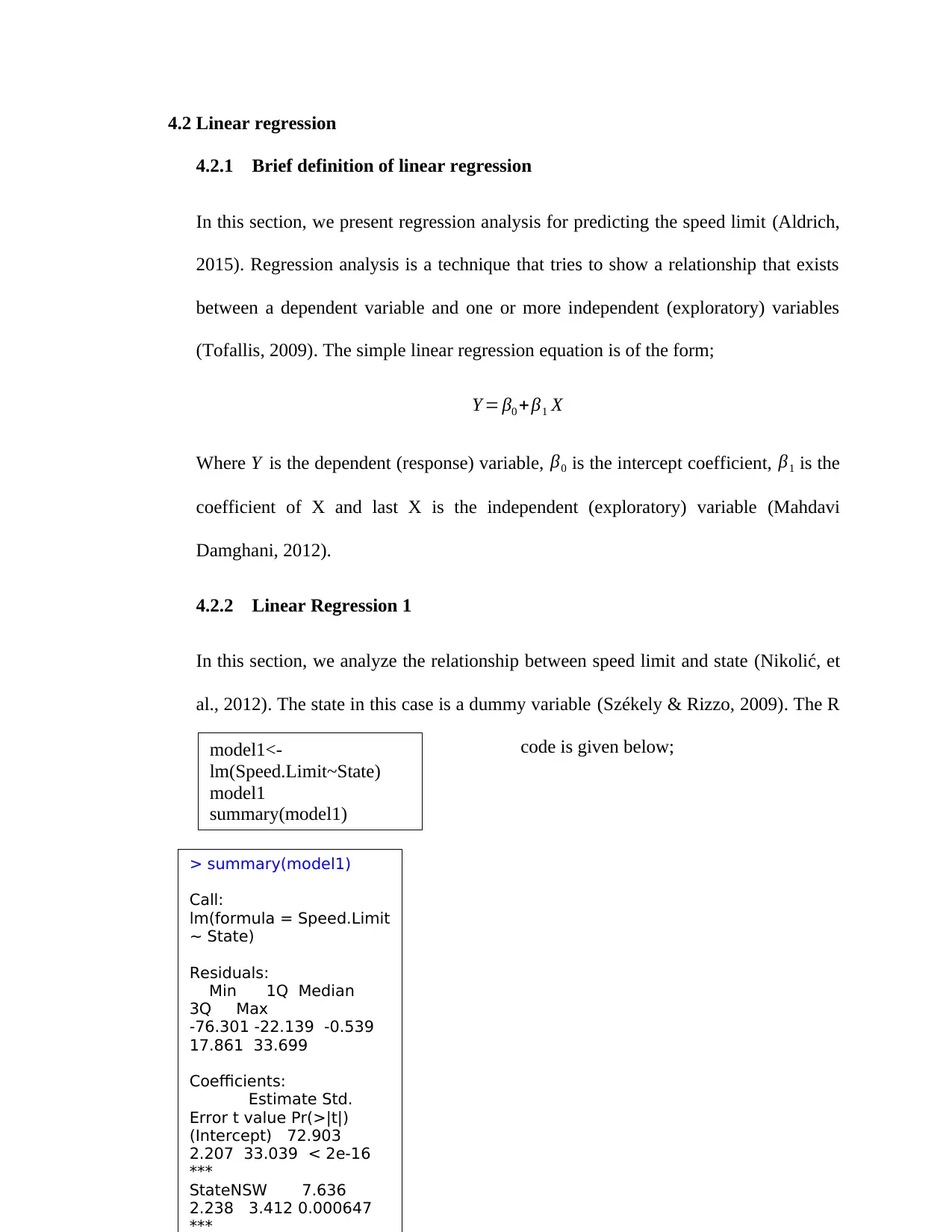
4.2.2 Linear Regression 1
In this section, we analyze the relationship between speed limit and state (Nikolić, et
al., 2012). The state in this case is a dummy variable (Székely & Rizzo, 2009). The R
code is given below;model1<-
lm(Speed.Limit~State)
model1
summary(model1)
> summary(model1)
Call:
lm(formula = Speed.Limit
~ State)
Residuals:
Min 1Q Median
3Q Max
-76.301 -22.139 -0.539
17.861 33.699
Coefficients:
Estimate Std.
Error t value Pr(>|t|)
(Intercept) 72.903
2.207 33.039 < 2e-16
***
StateNSW 7.636
2.238 3.412 0.000647
***
4.2.1 Brief definition of linear regression
In this section, we present regression analysis for predicting the speed limit (Aldrich,
2015). Regression analysis is a technique that tries to show a relationship that exists
between a dependent variable and one or more independent (exploratory) variables
(Tofallis, 2009). The simple linear regression equation is of the form;
Y = β0 +β1 X
Where Y is the dependent (response) variable, β0 is the intercept coefficient, β1 is the
coefficient of X and last X is the independent (exploratory) variable (Mahdavi
Damghani, 2012).
4.2.2 Linear Regression 1
In this section, we analyze the relationship between speed limit and state (Nikolić, et
al., 2012). The state in this case is a dummy variable (Székely & Rizzo, 2009). The R
code is given below;model1<-
lm(Speed.Limit~State)
model1
summary(model1)
> summary(model1)
Call:
lm(formula = Speed.Limit
~ State)
Residuals:
Min 1Q Median
3Q Max
-76.301 -22.139 -0.539
17.861 33.699
Coefficients:
Estimate Std.
Error t value Pr(>|t|)
(Intercept) 72.903
2.207 33.039 < 2e-16
***
StateNSW 7.636
2.238 3.412 0.000647
***
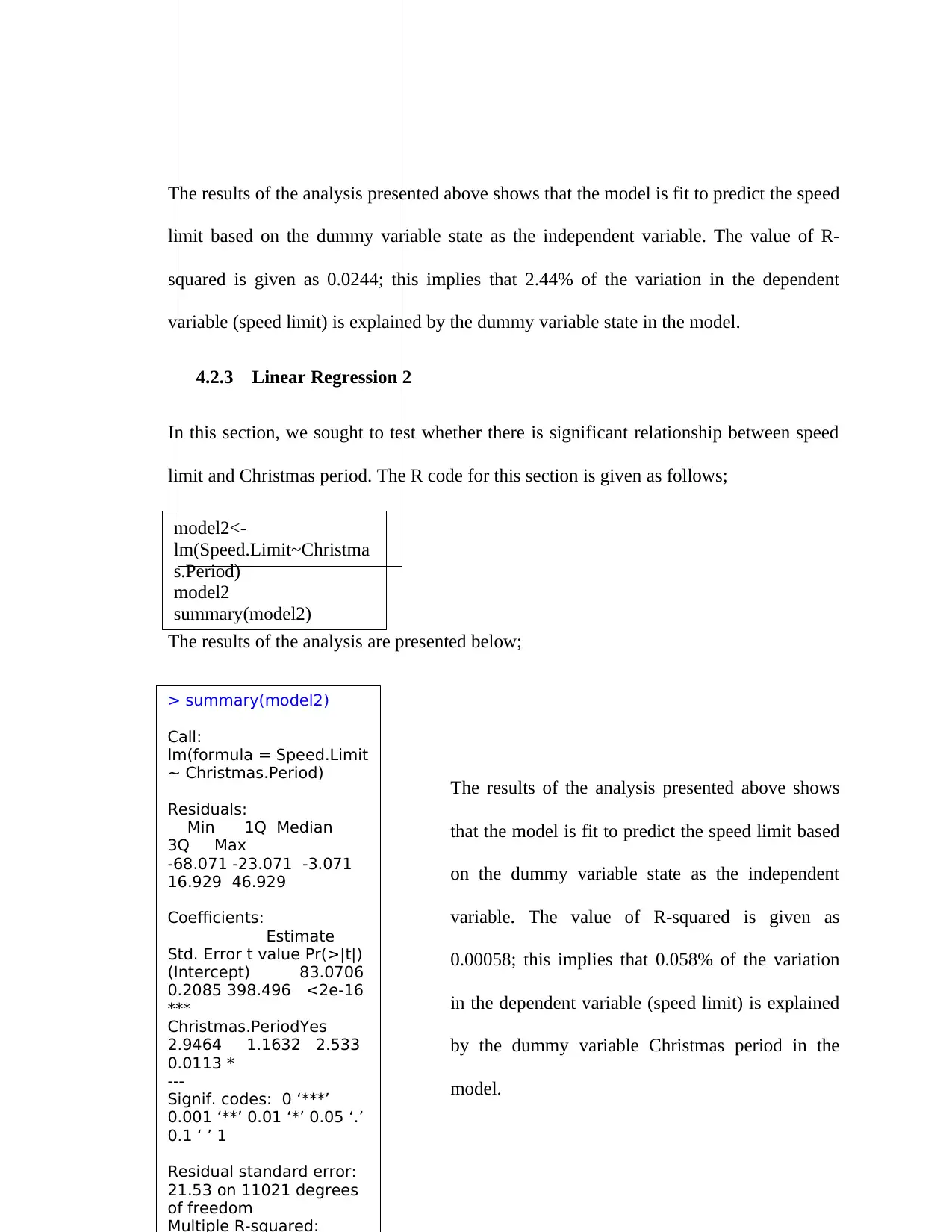
The results of the analysis presented above shows that the model is fit to predict the speed
limit based on the dummy variable state as the independent variable. The value of R-
squared is given as 0.0244; this implies that 2.44% of the variation in the dependent
variable (speed limit) is explained by the dummy variable state in the model.
4.2.3 Linear Regression 2
In this section, we sought to test whether there is significant relationship between speed
limit and Christmas period. The R code for this section is given as follows;
The results of the analysis are presented below;
The results of the analysis presented above shows
that the model is fit to predict the speed limit based
on the dummy variable state as the independent
variable. The value of R-squared is given as
0.00058; this implies that 0.058% of the variation
in the dependent variable (speed limit) is explained
by the dummy variable Christmas period in the
model.
> summary(model2)
Call:
lm(formula = Speed.Limit
~ Christmas.Period)
Residuals:
Min 1Q Median
3Q Max
-68.071 -23.071 -3.071
16.929 46.929
Coefficients:
Estimate
Std. Error t value Pr(>|t|)
(Intercept) 83.0706
0.2085 398.496 <2e-16
***
Christmas.PeriodYes
2.9464 1.1632 2.533
0.0113 *
---
Signif. codes: 0 ‘***’
0.001 ‘**’ 0.01 ‘*’ 0.05 ‘.’
0.1 ‘ ’ 1
Residual standard error:
21.53 on 11021 degrees
of freedom
Multiple R-squared:
model2<-
lm(Speed.Limit~Christma
s.Period)
model2
summary(model2)
⊘ This is a preview!⊘
Do you want full access?
Subscribe today to unlock all pages.
Trusted by 1+ million students worldwide
5. Conclusion
This study aimed at analyzing the trends in the fatalities in Australia. Results showed that
significant differences exist in the fatalities in the different states and territories within
Australia as well between the different gender groups. Results showed that female victims
tend to over-speed more as compared to the male victims.
6. Reflection
The study utilized various statistical techniques learnt in class to draw conclusions about the
data. Several statistical as well as machine learning algorithms were utilized. The study
shows the great importance of these techniques in helping to create meaningful decisions
from the dataset.
References
Aldrich, J., 2015. Fisher and Regression. Statistical Science, 20(4), p. 401–417.
Filipovych, R., Resnick, S. M. & Davatzikos, C., 2011. Semi-supervised Cluster Analysis of Imaging Data.
Journal of Neuro Image, 54(3), p. 2185–2197.
Frey, B. J. & Dueck, D., 2017. Clustering by Passing Messages Between Data Points. Journal of Science,
315 (5814), p. 972–976.
Mahdavi Damghani, B., 2012. The Misleading Value of Measured Correlation. Wilmott, 1(6), p. 64–73.
Meilă, M., 2013. Comparing Clusterings by the Variation of Information: Learning Theory and Kernel
Machines. Lecture Notes in Computer Science, Volume 2777, p. 173–187.
Nikolić, D., Muresan, R., Feng, W. & Singer, W., 2012. Scaled correlation analysis: a better way to
compute a cross-correlogram. European Journal of Neuroscience, 35(5), p. 1–21.
Székely, G. J. & Rizzo, M. L., 2009. Brownian distance covariance. Annals of Applied Statistics, 3(4), p.
1233–1303.
Tofallis, C., 2009. Least Squares Percentage Regression. Journal of Modern Applied Statistical Methods,
7(5), p. 526–534.
Paraphrase This Document
Need a fresh take? Get an instant paraphrase of this document with our AI Paraphraser
Appendix
R codes
fatalities<-read.csv("C:\\Users\\Documents\\fatalities.csv")
str(fatalities)
attach(fatalities)
install.packages("cluster")
library(cluster)
summary(fatalities$Age, fatalities$Age>0)
boxplot(Age, ylab="Age",
main="Boxplot of Age", col="chartreuse1")
summary(fatalities$Speed.Limit)
hist(Speed.Limit, xlab="Speed Limit", ylab="Frequency",
main="Histogram of Speed Limit", col="darkslategray1")
t.test(Speed.Limit~Gender)
slices <- c(84.50, 82.66)
lbls <- c("Female", "Male")
pie(slices, labels = lbls, main="Pie Chart of average speed limit by gender")
barplot(slices,names.arg=lbls,xlab="Gender",ylab="Average speed limit"
,col="blue", main="Speed limit chart",border="red")
install.packages("plyr")
library(plyr)
ddply(fatalities,~State,summarise,mean=mean(Speed.Limit))
slices <- c(72.90, 80.54, 96.30, 82.14, 84.70, 84.67, 82.90, 86.77)
lbls <- c("ACT", "NSW", "NT", "QLD", "SA", "TAS", "VIC", "WA")
barplot(slices,names.arg=lbls,xlab="State",ylab="Average speed limit"
,col="green", main="Speed limit chart",border="red")
model1<-lm(Speed.Limit~State)
model1
summary(model1)
anova(model1)
model2<-lm(Speed.Limit~Christmas.Period)
model2
summary(model2)
anova(model2)
⊘ This is a preview!⊘
Do you want full access?
Subscribe today to unlock all pages.
Trusted by 1+ million students worldwide
1 out of 12
Related Documents


![Credit Scoring Model Development and Analysis - [Course Name]](/_next/image/?url=https%3A%2F%2Fdesklib.com%2Fmedia%2Fimages%2Fxd%2F3b3e7431b5e5468f919174fbcc150dc9.jpg&w=256&q=75)


Your All-in-One AI-Powered Toolkit for Academic Success.
+13062052269
info@desklib.com
Available 24*7 on WhatsApp / Email
![[object Object]](/_next/static/media/star-bottom.7253800d.svg)
Unlock your academic potential
Copyright © 2020–2025 A2Z Services. All Rights Reserved. Developed and managed by ZUCOL.