Analysis of Retail Surge's Product Categories: Profit, COGS, Payment Methods, and Customer Attitudes | Desklib
VerifiedAdded on 2023/06/04
|26
|4312
|494
AI Summary
This report analyses Retail Surge's product categories that generate the most profit, have the highest cost of goods, payment methods, and customer attitudes. ANOVA, t-test, and Chi-Square tests were used for analysis. The report provides insights on the product categories that generate the most profit and have the highest cost of goods. It also analyses the payment methods and customer attitudes, including the association between user groups and customer attitudes and gender and customer attitudes.
Contribute Materials
Your contribution can guide someone’s learning journey. Share your
documents today.
Business Statistics
Student Name:
Instructor Name:
Course Number:
17 September 2018
Student Name:
Instructor Name:
Course Number:
17 September 2018
Secure Best Marks with AI Grader
Need help grading? Try our AI Grader for instant feedback on your assignments.
Table of Contents
List of tables....................................................................................................................................2
Introduction......................................................................................................................................3
Problem definition and business intelligence required....................................................................3
Results of the selected analytics methods and technical analysis....................................................4
Which product categories are making the most profit?...............................................................4
Which product category costs the most (COGS)?.......................................................................6
Is there a difference in payments methods?.................................................................................7
Are there any differences in the user groups on all of the customer attitudes?...........................8
Are there any differences in gender on all of the customer attitudes?.........................................9
Discussion of the results and recommendations............................................................................10
Recommendations..........................................................................................................................10
References......................................................................................................................................11
Appendix........................................................................................................................................12
List of tables
Table 1: Descriptive Statistics.........................................................................................................5
Table 2: Test of Homogeneity of Variances....................................................................................5
Table 3: ANOVA.............................................................................................................................5
Table 4: Descriptive Statistics.........................................................................................................6
Table 5: ANOVA.............................................................................................................................7
Table 6: t-Test: Two-Sample Assuming Equal Variances..............................................................7
Table 7: Chi-Square test of association (user group and customer attitudes)..................................8
Table 8: Chi-Square test of association (gender and customer attitudes)........................................9
Introduction
This report is about an online retail company called, Retail Surge. The company has its
business divided into several areas including Boy’s, Men’s, Girl’s, Women’s and
Customisation. The company’s product range includes clothing, shoes, sporting equipment
and accessories. This report seeks to analyse and understand the product categories that
generate more income to the company. It also sought to understand the product categories
that had the largest cost of goods. Lastly, the study looked at the association between
gender/website user groups and customer attitudes.
Problem definition and business intelligence required
This study sought to answer the following research questions.
Which product categories are making the most profit?
To answer this research question, analysis of variance (ANOVA) was employed
(Hinkelmann & Kempthorne, 2008). ANOVA is used to analyse variation in the means of
groups that are more than 2. Since the product categories were more than 2, ANOVA was
the most ideal test to be used.
Which product category costs the most (COGS)?
Again to answer this research question, analysis of variance (ANOVA) was employed
(Hinkelmann & Kempthorne, 2008). ANOVA is used to analyse variation in the means of
groups that are more than 2 (Gelman, 2005). Since the product categories were more than
2, ANOVA was the most ideal test to be used.
Is there a difference in payments methods?
Answering this research question required the use of t-test is that test that helps compare
Secure Best Marks with AI Grader
Need help grading? Try our AI Grader for instant feedback on your assignments.
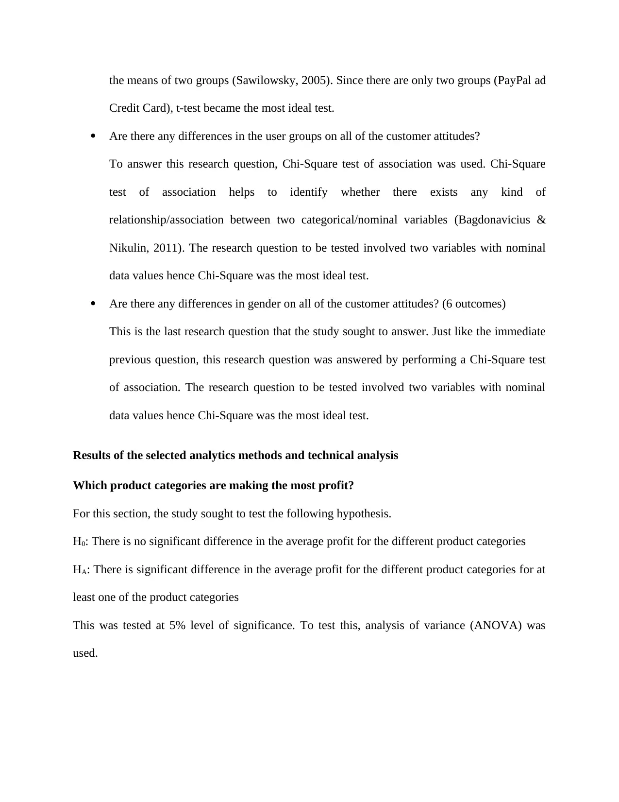
the means of two groups (Sawilowsky, 2005). Since there are only two groups (PayPal ad
Credit Card), t-test became the most ideal test.
Are there any differences in the user groups on all of the customer attitudes?
To answer this research question, Chi-Square test of association was used. Chi-Square
test of association helps to identify whether there exists any kind of
relationship/association between two categorical/nominal variables (Bagdonavicius &
Nikulin, 2011). The research question to be tested involved two variables with nominal
data values hence Chi-Square was the most ideal test.
Are there any differences in gender on all of the customer attitudes? (6 outcomes)
This is the last research question that the study sought to answer. Just like the immediate
previous question, this research question was answered by performing a Chi-Square test
of association. The research question to be tested involved two variables with nominal
data values hence Chi-Square was the most ideal test.
Results of the selected analytics methods and technical analysis
Which product categories are making the most profit?
For this section, the study sought to test the following hypothesis.
H0: There is no significant difference in the average profit for the different product categories
HA: There is significant difference in the average profit for the different product categories for at
least one of the product categories
This was tested at 5% level of significance. To test this, analysis of variance (ANOVA) was
used.
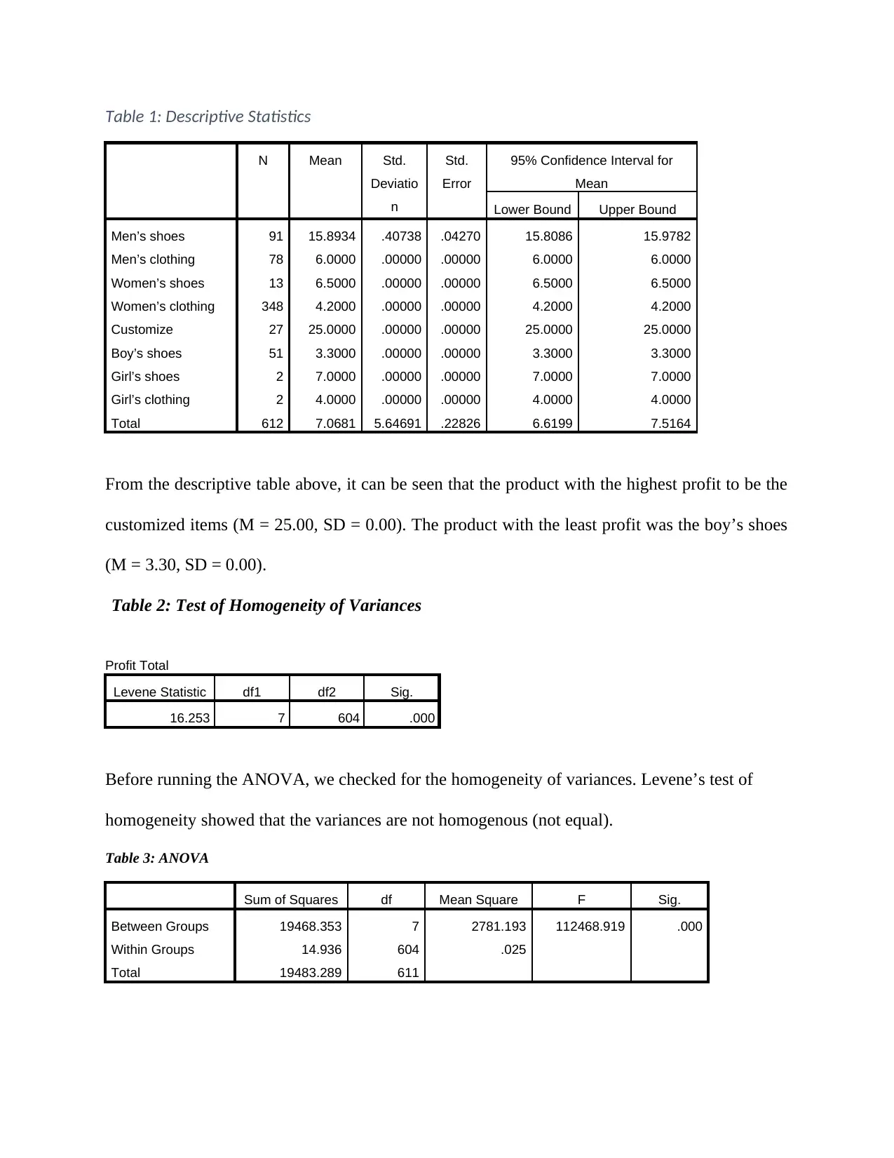
Table 1: Descriptive Statistics
N Mean Std.
Deviatio
n
Std.
Error
95% Confidence Interval for
Mean
Lower Bound Upper Bound
Men’s shoes 91 15.8934 .40738 .04270 15.8086 15.9782
Men’s clothing 78 6.0000 .00000 .00000 6.0000 6.0000
Women’s shoes 13 6.5000 .00000 .00000 6.5000 6.5000
Women’s clothing 348 4.2000 .00000 .00000 4.2000 4.2000
Customize 27 25.0000 .00000 .00000 25.0000 25.0000
Boy’s shoes 51 3.3000 .00000 .00000 3.3000 3.3000
Girl’s shoes 2 7.0000 .00000 .00000 7.0000 7.0000
Girl’s clothing 2 4.0000 .00000 .00000 4.0000 4.0000
Total 612 7.0681 5.64691 .22826 6.6199 7.5164
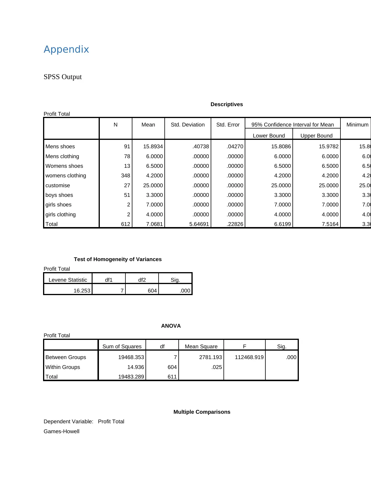
From the descriptive table above, it can be seen that the product with the highest profit to be the
customized items (M = 25.00, SD = 0.00). The product with the least profit was the boy’s shoes
(M = 3.30, SD = 0.00).
Table 2: Test of Homogeneity of Variances
Profit Total
Levene Statistic df1 df2 Sig.
16.253 7 604 .000
Before running the ANOVA, we checked for the homogeneity of variances. Levene’s test of
homogeneity showed that the variances are not homogenous (not equal).
Table 3: ANOVA
Sum of Squares df Mean Square F Sig.
Between Groups 19468.353 7 2781.193 112468.919 .000
Within Groups 14.936 604 .025
Total 19483.289 611
N Mean Std.
Deviatio
n
Std.
Error
95% Confidence Interval for
Mean
Lower Bound Upper Bound
Men’s shoes 91 15.8934 .40738 .04270 15.8086 15.9782
Men’s clothing 78 6.0000 .00000 .00000 6.0000 6.0000
Women’s shoes 13 6.5000 .00000 .00000 6.5000 6.5000
Women’s clothing 348 4.2000 .00000 .00000 4.2000 4.2000
Customize 27 25.0000 .00000 .00000 25.0000 25.0000
Boy’s shoes 51 3.3000 .00000 .00000 3.3000 3.3000
Girl’s shoes 2 7.0000 .00000 .00000 7.0000 7.0000
Girl’s clothing 2 4.0000 .00000 .00000 4.0000 4.0000
Total 612 7.0681 5.64691 .22826 6.6199 7.5164
From the descriptive table above, it can be seen that the product with the highest profit to be the
customized items (M = 25.00, SD = 0.00). The product with the least profit was the boy’s shoes
(M = 3.30, SD = 0.00).
Table 2: Test of Homogeneity of Variances
Profit Total
Levene Statistic df1 df2 Sig.
16.253 7 604 .000
Before running the ANOVA, we checked for the homogeneity of variances. Levene’s test of
homogeneity showed that the variances are not homogenous (not equal).
Table 3: ANOVA
Sum of Squares df Mean Square F Sig.
Between Groups 19468.353 7 2781.193 112468.919 .000
Within Groups 14.936 604 .025
Total 19483.289 611
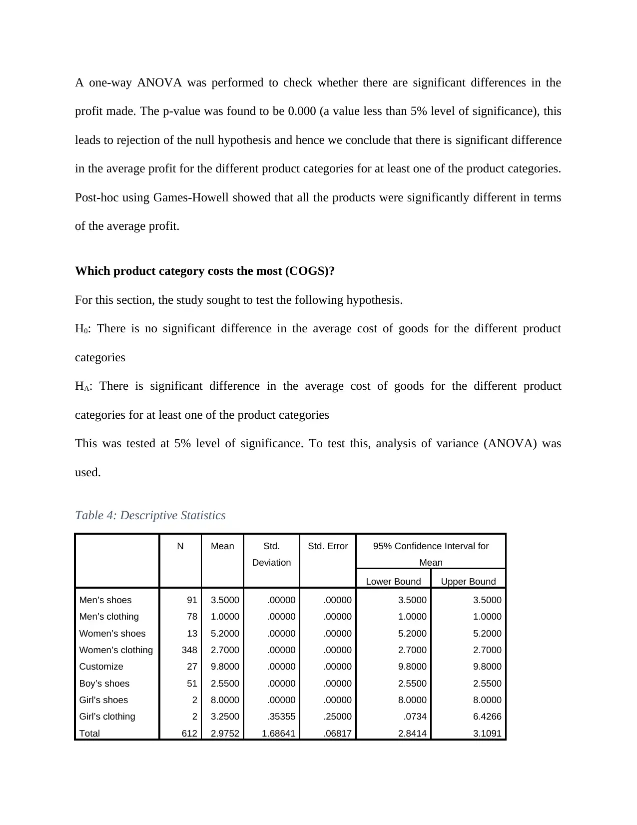
A one-way ANOVA was performed to check whether there are significant differences in the
profit made. The p-value was found to be 0.000 (a value less than 5% level of significance), this
leads to rejection of the null hypothesis and hence we conclude that there is significant difference
in the average profit for the different product categories for at least one of the product categories.
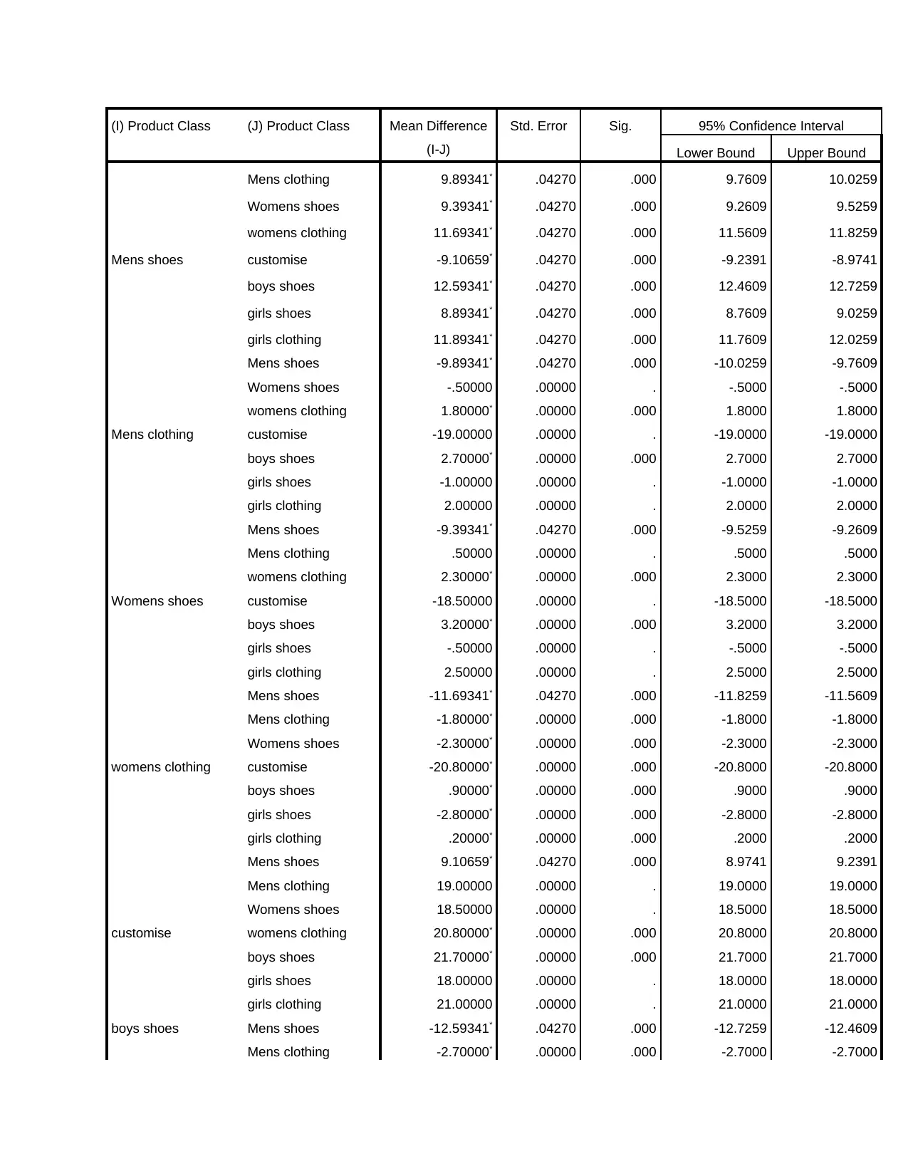
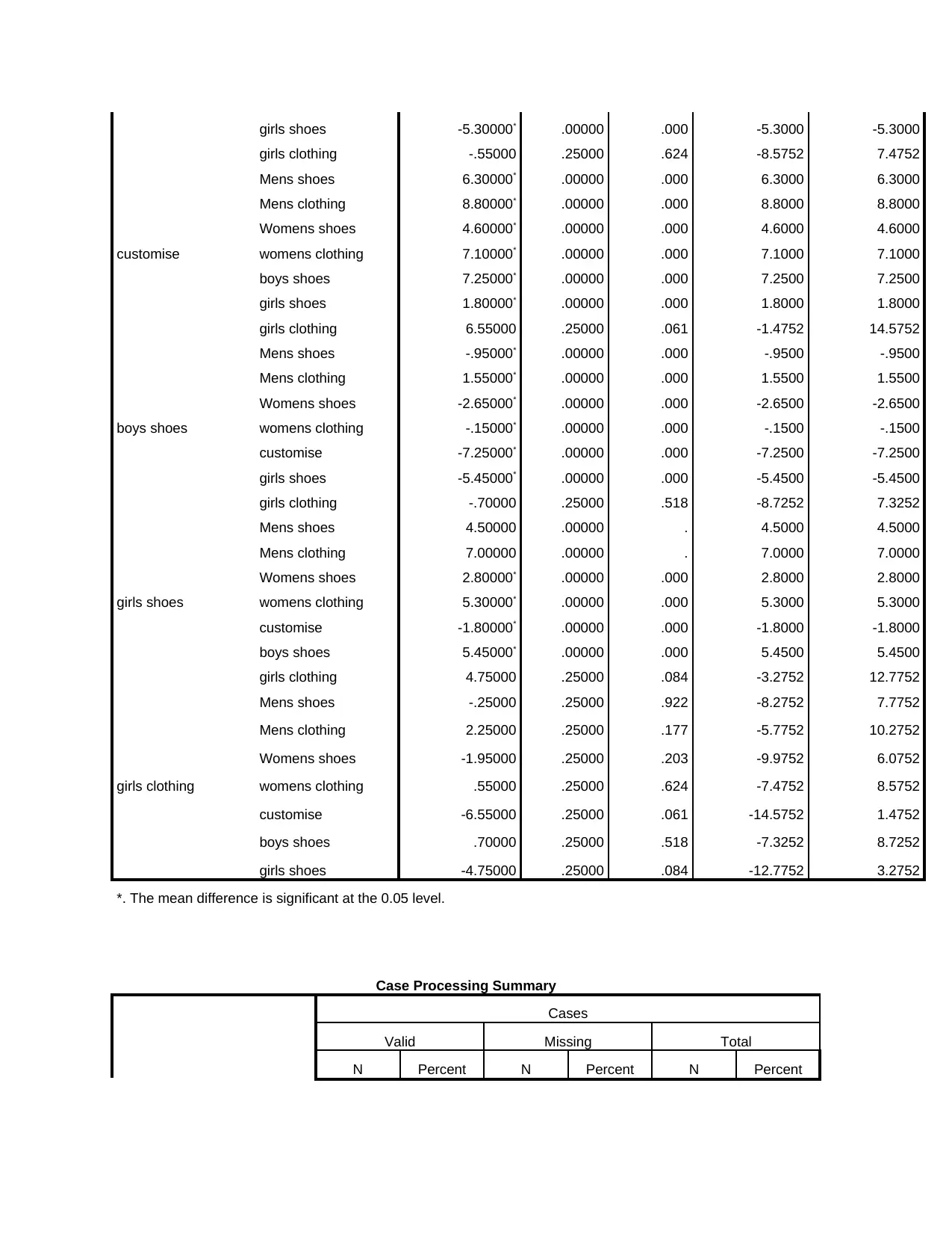
Post-hoc using Games-Howell showed that all the products were significantly different in terms
of the average profit.
Which product category costs the most (COGS)?
For this section, the study sought to test the following hypothesis.
H0: There is no significant difference in the average cost of goods for the different product
categories
HA: There is significant difference in the average cost of goods for the different product
categories for at least one of the product categories
This was tested at 5% level of significance. To test this, analysis of variance (ANOVA) was
used.
Table 4: Descriptive Statistics
N Mean Std.
Deviation
Std. Error 95% Confidence Interval for
Mean
Lower Bound Upper Bound
Men’s shoes 91 3.5000 .00000 .00000 3.5000 3.5000
Men’s clothing 78 1.0000 .00000 .00000 1.0000 1.0000
Women’s shoes 13 5.2000 .00000 .00000 5.2000 5.2000
Women’s clothing 348 2.7000 .00000 .00000 2.7000 2.7000
Customize 27 9.8000 .00000 .00000 9.8000 9.8000
Boy’s shoes 51 2.5500 .00000 .00000 2.5500 2.5500
Girl’s shoes 2 8.0000 .00000 .00000 8.0000 8.0000
Girl’s clothing 2 3.2500 .35355 .25000 .0734 6.4266
Total 612 2.9752 1.68641 .06817 2.8414 3.1091
profit made. The p-value was found to be 0.000 (a value less than 5% level of significance), this
leads to rejection of the null hypothesis and hence we conclude that there is significant difference
in the average profit for the different product categories for at least one of the product categories.
Post-hoc using Games-Howell showed that all the products were significantly different in terms
of the average profit.
Which product category costs the most (COGS)?
For this section, the study sought to test the following hypothesis.
H0: There is no significant difference in the average cost of goods for the different product
categories
HA: There is significant difference in the average cost of goods for the different product
categories for at least one of the product categories
This was tested at 5% level of significance. To test this, analysis of variance (ANOVA) was
used.
Table 4: Descriptive Statistics
N Mean Std.
Deviation
Std. Error 95% Confidence Interval for
Mean
Lower Bound Upper Bound
Men’s shoes 91 3.5000 .00000 .00000 3.5000 3.5000
Men’s clothing 78 1.0000 .00000 .00000 1.0000 1.0000
Women’s shoes 13 5.2000 .00000 .00000 5.2000 5.2000
Women’s clothing 348 2.7000 .00000 .00000 2.7000 2.7000
Customize 27 9.8000 .00000 .00000 9.8000 9.8000
Boy’s shoes 51 2.5500 .00000 .00000 2.5500 2.5500
Girl’s shoes 2 8.0000 .00000 .00000 8.0000 8.0000
Girl’s clothing 2 3.2500 .35355 .25000 .0734 6.4266
Total 612 2.9752 1.68641 .06817 2.8414 3.1091
Paraphrase This Document
Need a fresh take? Get an instant paraphrase of this document with our AI Paraphraser
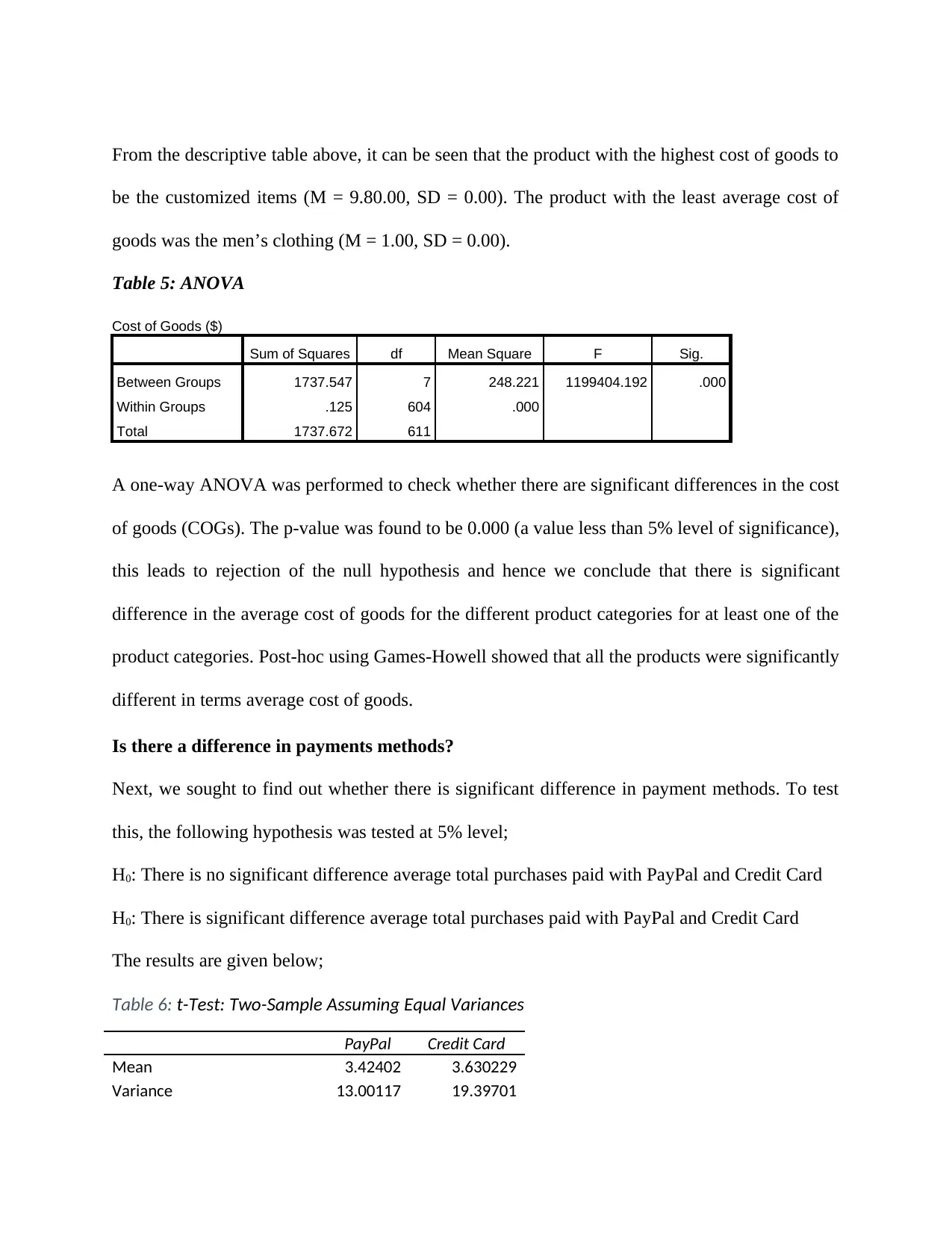
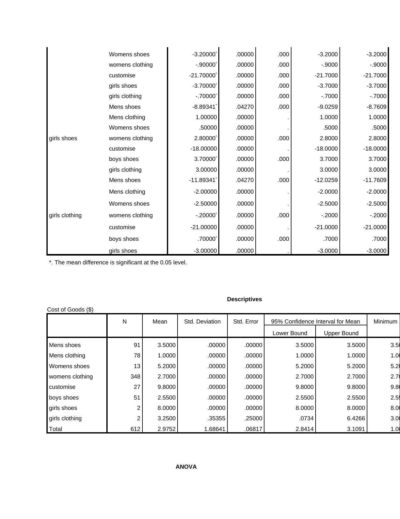
From the descriptive table above, it can be seen that the product with the highest cost of goods to
be the customized items (M = 9.80.00, SD = 0.00). The product with the least average cost of
goods was the men’s clothing (M = 1.00, SD = 0.00).
Table 5: ANOVA
Cost of Goods ($)
Sum of Squares df Mean Square F Sig.
Between Groups 1737.547 7 248.221 1199404.192 .000
Within Groups .125 604 .000
Total 1737.672 611
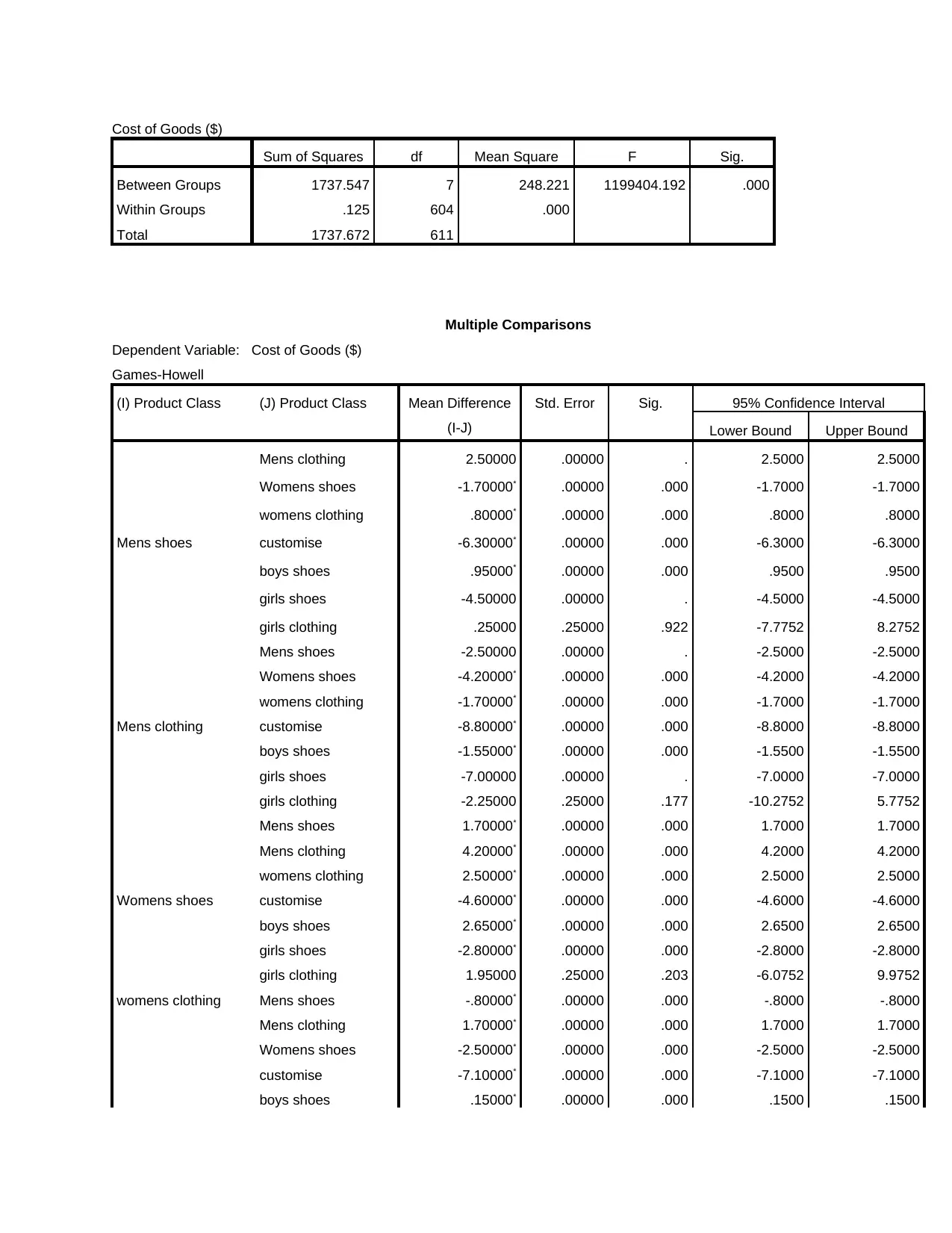
A one-way ANOVA was performed to check whether there are significant differences in the cost
of goods (COGs). The p-value was found to be 0.000 (a value less than 5% level of significance),
this leads to rejection of the null hypothesis and hence we conclude that there is significant
difference in the average cost of goods for the different product categories for at least one of the
product categories. Post-hoc using Games-Howell showed that all the products were significantly
different in terms average cost of goods.
Is there a difference in payments methods?
Next, we sought to find out whether there is significant difference in payment methods. To test
this, the following hypothesis was tested at 5% level;
H0: There is no significant difference average total purchases paid with PayPal and Credit Card
H0: There is significant difference average total purchases paid with PayPal and Credit Card
The results are given below;
Table 6: t-Test: Two-Sample Assuming Equal Variances
PayPal Credit Card
Mean 3.42402 3.630229
Variance 13.00117 19.39701
be the customized items (M = 9.80.00, SD = 0.00). The product with the least average cost of
goods was the men’s clothing (M = 1.00, SD = 0.00).
Table 5: ANOVA
Cost of Goods ($)
Sum of Squares df Mean Square F Sig.
Between Groups 1737.547 7 248.221 1199404.192 .000
Within Groups .125 604 .000
Total 1737.672 611
A one-way ANOVA was performed to check whether there are significant differences in the cost
of goods (COGs). The p-value was found to be 0.000 (a value less than 5% level of significance),
this leads to rejection of the null hypothesis and hence we conclude that there is significant
difference in the average cost of goods for the different product categories for at least one of the
product categories. Post-hoc using Games-Howell showed that all the products were significantly
different in terms average cost of goods.
Is there a difference in payments methods?
Next, we sought to find out whether there is significant difference in payment methods. To test
this, the following hypothesis was tested at 5% level;
H0: There is no significant difference average total purchases paid with PayPal and Credit Card
H0: There is significant difference average total purchases paid with PayPal and Credit Card
The results are given below;
Table 6: t-Test: Two-Sample Assuming Equal Variances
PayPal Credit Card
Mean 3.42402 3.630229
Variance 13.00117 19.39701
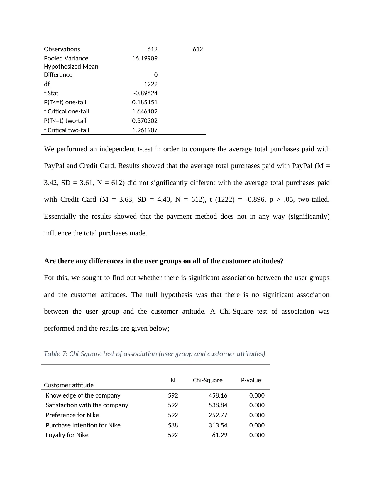
Observations 612 612
Pooled Variance 16.19909
Hypothesized Mean
Difference 0
df 1222
t Stat -0.89624
P(T<=t) one-tail 0.185151
t Critical one-tail 1.646102
P(T<=t) two-tail 0.370302
t Critical two-tail 1.961907
We performed an independent t-test in order to compare the average total purchases paid with
PayPal and Credit Card. Results showed that the average total purchases paid with PayPal (M =
3.42, SD = 3.61, N = 612) did not significantly different with the average total purchases paid
with Credit Card (M = 3.63, SD = 4.40, N = 612), t (1222) = -0.896, p > .05, two-tailed.
Essentially the results showed that the payment method does not in any way (significantly)
influence the total purchases made.
Are there any differences in the user groups on all of the customer attitudes?
For this, we sought to find out whether there is significant association between the user groups
and the customer attitudes. The null hypothesis was that there is no significant association
between the user group and the customer attitude. A Chi-Square test of association was
performed and the results are given below;
Table 7: Chi-Square test of association (user group and customer attitudes)
Customer attitude N Chi-Square P-value
Knowledge of the company 592 458.16 0.000
Satisfaction with the company 592 538.84 0.000
Preference for Nike 592 252.77 0.000
Purchase Intention for Nike 588 313.54 0.000
Loyalty for Nike 592 61.29 0.000
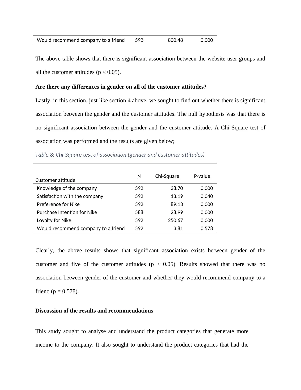
Would recommend company to a friend 592 800.48 0.000
The above table shows that there is significant association between the website user groups and
all the customer attitudes (p < 0.05).
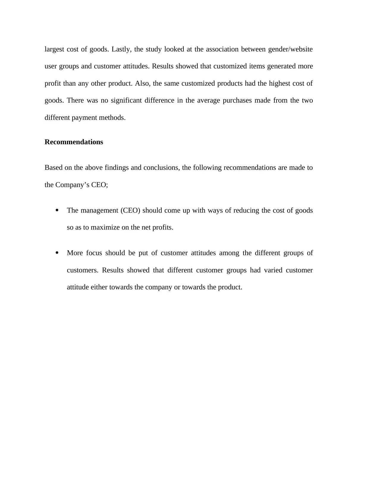
Are there any differences in gender on all of the customer attitudes?
Lastly, in this section, just like section 4 above, we sought to find out whether there is significant
association between the gender and the customer attitudes. The null hypothesis was that there is
no significant association between the gender and the customer attitude. A Chi-Square test of
association was performed and the results are given below;
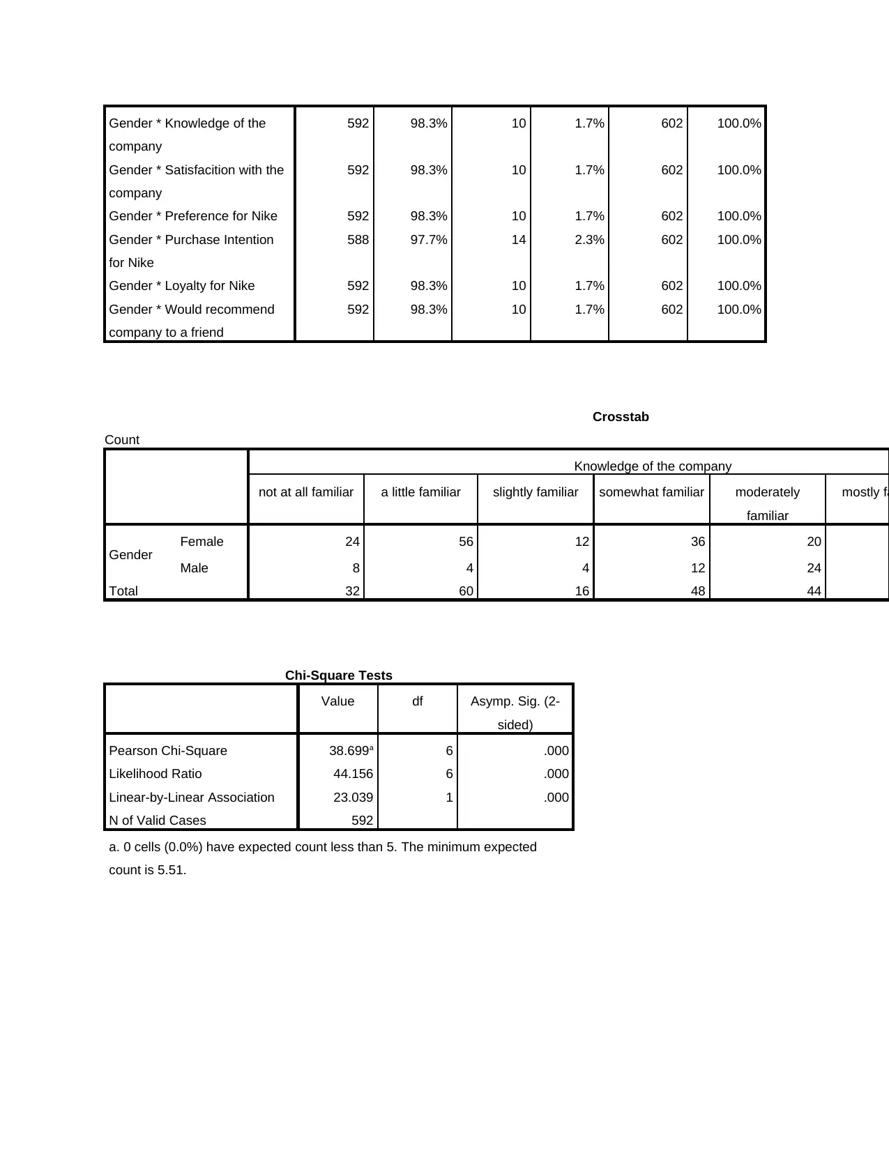
Table 8: Chi-Square test of association (gender and customer attitudes)
Customer attitude N Chi-Square P-value
Knowledge of the company 592 38.70 0.000
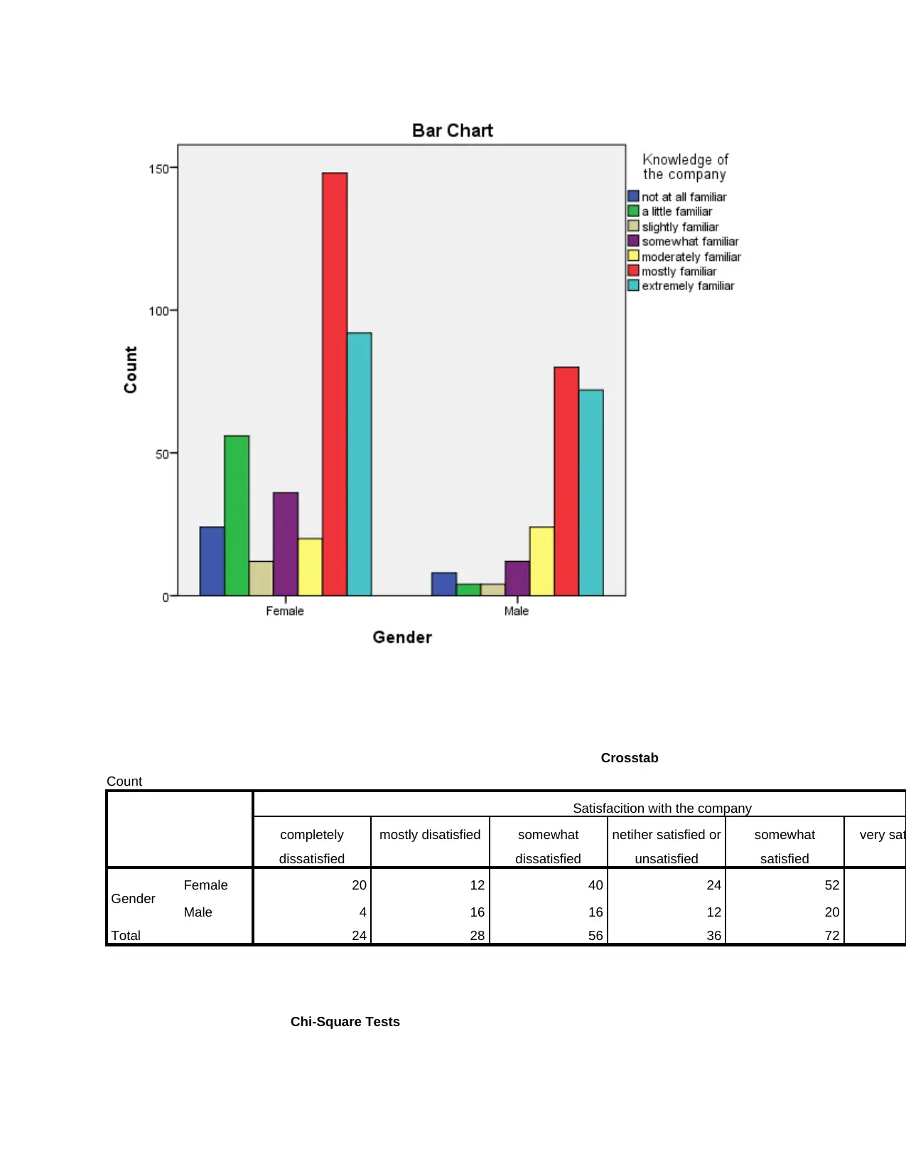
Satisfaction with the company 592 13.19 0.040
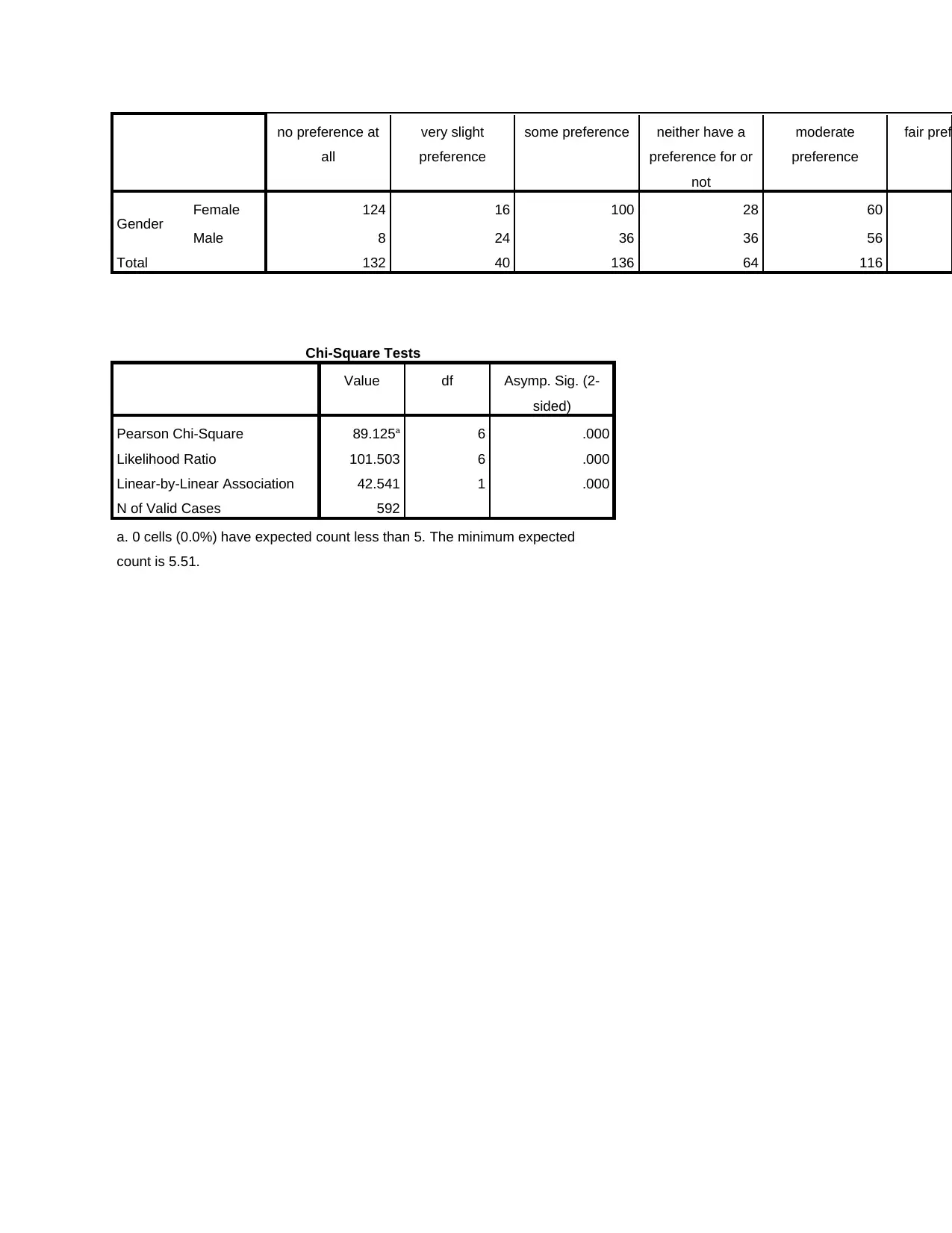
Preference for Nike 592 89.13 0.000
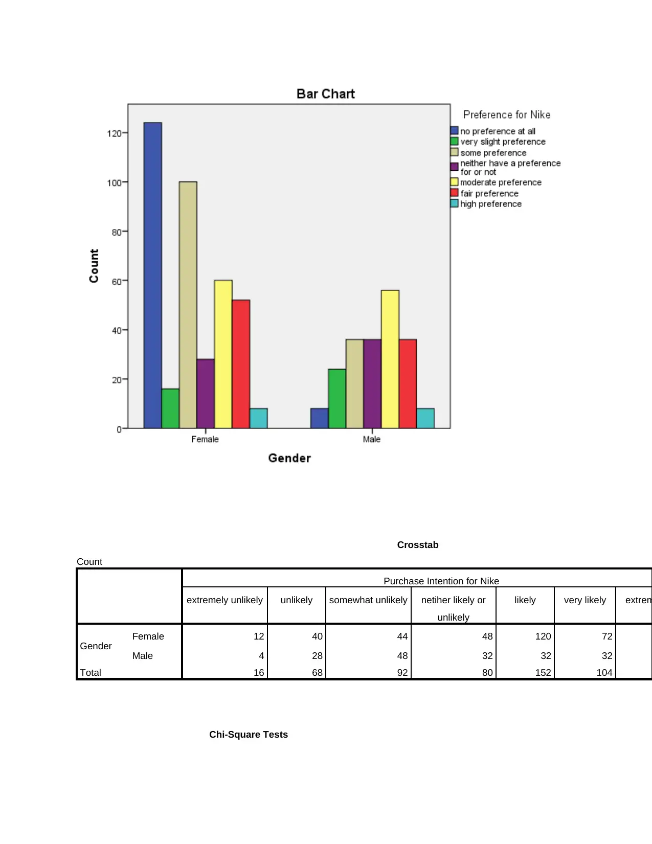
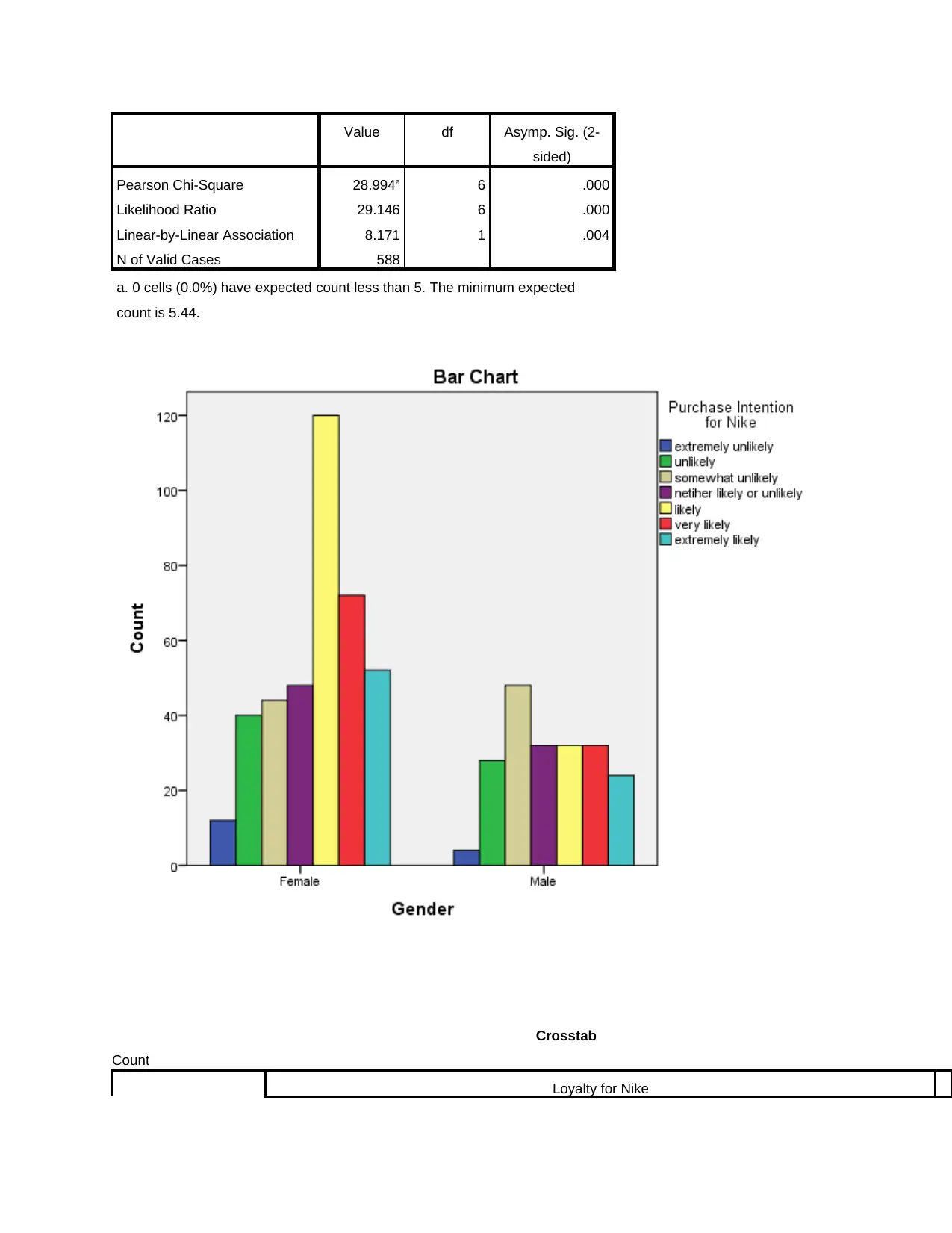
Purchase Intention for Nike 588 28.99 0.000
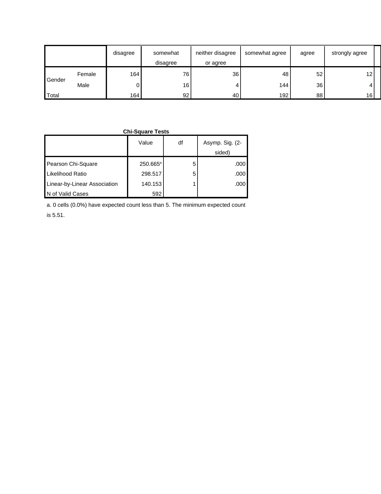
Loyalty for Nike 592 250.67 0.000
Would recommend company to a friend 592 3.81 0.578
Clearly, the above results shows that significant association exists between gender of the
customer and five of the customer attitudes (p < 0.05). Results showed that there was no
association between gender of the customer and whether they would recommend company to a
friend (p = 0.578).
Discussion of the results and recommendations
This study sought to analyse and understand the product categories that generate more
income to the company. It also sought to understand the product categories that had the
The above table shows that there is significant association between the website user groups and
all the customer attitudes (p < 0.05).
Are there any differences in gender on all of the customer attitudes?
Lastly, in this section, just like section 4 above, we sought to find out whether there is significant
association between the gender and the customer attitudes. The null hypothesis was that there is
no significant association between the gender and the customer attitude. A Chi-Square test of
association was performed and the results are given below;
Table 8: Chi-Square test of association (gender and customer attitudes)
Customer attitude N Chi-Square P-value
Knowledge of the company 592 38.70 0.000
Satisfaction with the company 592 13.19 0.040
Preference for Nike 592 89.13 0.000
Purchase Intention for Nike 588 28.99 0.000
Loyalty for Nike 592 250.67 0.000
Would recommend company to a friend 592 3.81 0.578
Clearly, the above results shows that significant association exists between gender of the
customer and five of the customer attitudes (p < 0.05). Results showed that there was no
association between gender of the customer and whether they would recommend company to a
friend (p = 0.578).
Discussion of the results and recommendations
This study sought to analyse and understand the product categories that generate more
income to the company. It also sought to understand the product categories that had the
Secure Best Marks with AI Grader
Need help grading? Try our AI Grader for instant feedback on your assignments.
largest cost of goods. Lastly, the study looked at the association between gender/website
user groups and customer attitudes. Results showed that customized items generated more
profit than any other product. Also, the same customized products had the highest cost of
goods. There was no significant difference in the average purchases made from the two
different payment methods.
Recommendations
Based on the above findings and conclusions, the following recommendations are made to
the Company’s CEO;
The management (CEO) should come up with ways of reducing the cost of goods
so as to maximize on the net profits.
More focus should be put of customer attitudes among the different groups of
customers. Results showed that different customer groups had varied customer
attitude either towards the company or towards the product.
References
Bagdonavicius, V., & Nikulin, M. S. (2011). Chi-squared goodness-of-fit test for right censored
data. The International Journal of Applied Mathematics and Statistics, 30–50.
Gelman, A. (2005). Analysis of variance? Why it is more important than ever. The Annals of
Statistics, 33(5), 1–53. doi:10.1214/009053604000001048
Hinkelmann, K., & Kempthorne, O. (2008). Design and Analysis of Experiments. Journal of the
Royal Statistical Society, 251 (5), 251–276.
Sawilowsky, S. (2005). Misconceptions Leading to Choosing the t Test Over The Wilcoxon
Mann–Whitney Test for Shift in Location Parameter. Journal of Modern Applied
Statistical Methods, 4(2), 598–600.
Appendix
SPSS Output
Descriptives
Profit Total
N Mean Std. Deviation Std. Error 95% Confidence Interval for Mean Minimum
Lower Bound Upper Bound
Mens shoes 91 15.8934 .40738 .04270 15.8086 15.9782 15.80
Mens clothing 78 6.0000 .00000 .00000 6.0000 6.0000 6.00
Womens shoes 13 6.5000 .00000 .00000 6.5000 6.5000 6.50
womens clothing 348 4.2000 .00000 .00000 4.2000 4.2000 4.20
customise 27 25.0000 .00000 .00000 25.0000 25.0000 25.00
boys shoes 51 3.3000 .00000 .00000 3.3000 3.3000 3.30
girls shoes 2 7.0000 .00000 .00000 7.0000 7.0000 7.00
girls clothing 2 4.0000 .00000 .00000 4.0000 4.0000 4.00
Total 612 7.0681 5.64691 .22826 6.6199 7.5164 3.30
Test of Homogeneity of Variances
Profit Total
Levene Statistic df1 df2 Sig.
16.253 7 604 .000
ANOVA
Profit Total
Sum of Squares df Mean Square F Sig.
Between Groups 19468.353 7 2781.193 112468.919 .000
Within Groups 14.936 604 .025
Total 19483.289 611
Multiple Comparisons
Dependent Variable: Profit Total
Games-Howell
Paraphrase This Document
Need a fresh take? Get an instant paraphrase of this document with our AI Paraphraser
(I) Product Class (J) Product Class Mean Difference
(I-J)
Std. Error Sig. 95% Confidence Interval
Lower Bound Upper Bound
Mens shoes
Mens clothing 9.89341* .04270 .000 9.7609 10.0259
Womens shoes 9.39341* .04270 .000 9.2609 9.5259
womens clothing 11.69341* .04270 .000 11.5609 11.8259
customise -9.10659* .04270 .000 -9.2391 -8.9741
boys shoes 12.59341* .04270 .000 12.4609 12.7259
girls shoes 8.89341* .04270 .000 8.7609 9.0259
girls clothing 11.89341* .04270 .000 11.7609 12.0259
Mens clothing
Mens shoes -9.89341* .04270 .000 -10.0259 -9.7609
Womens shoes -.50000 .00000 . -.5000 -.5000
womens clothing 1.80000* .00000 .000 1.8000 1.8000
customise -19.00000 .00000 . -19.0000 -19.0000
boys shoes 2.70000* .00000 .000 2.7000 2.7000
girls shoes -1.00000 .00000 . -1.0000 -1.0000
girls clothing 2.00000 .00000 . 2.0000 2.0000
Womens shoes
Mens shoes -9.39341* .04270 .000 -9.5259 -9.2609
Mens clothing .50000 .00000 . .5000 .5000
womens clothing 2.30000* .00000 .000 2.3000 2.3000
customise -18.50000 .00000 . -18.5000 -18.5000
boys shoes 3.20000* .00000 .000 3.2000 3.2000
girls shoes -.50000 .00000 . -.5000 -.5000
girls clothing 2.50000 .00000 . 2.5000 2.5000
womens clothing
Mens shoes -11.69341* .04270 .000 -11.8259 -11.5609
Mens clothing -1.80000* .00000 .000 -1.8000 -1.8000
Womens shoes -2.30000* .00000 .000 -2.3000 -2.3000
customise -20.80000* .00000 .000 -20.8000 -20.8000
boys shoes .90000* .00000 .000 .9000 .9000
girls shoes -2.80000* .00000 .000 -2.8000 -2.8000
girls clothing .20000* .00000 .000 .2000 .2000
customise
Mens shoes 9.10659* .04270 .000 8.9741 9.2391
Mens clothing 19.00000 .00000 . 19.0000 19.0000
Womens shoes 18.50000 .00000 . 18.5000 18.5000
womens clothing 20.80000* .00000 .000 20.8000 20.8000
boys shoes 21.70000* .00000 .000 21.7000 21.7000
girls shoes 18.00000 .00000 . 18.0000 18.0000
girls clothing 21.00000 .00000 . 21.0000 21.0000
boys shoes Mens shoes -12.59341* .04270 .000 -12.7259 -12.4609
Mens clothing -2.70000* .00000 .000 -2.7000 -2.7000
Womens shoes -3.20000* .00000 .000 -3.2000 -3.2000
womens clothing -.90000* .00000 .000 -.9000 -.9000
customise -21.70000* .00000 .000 -21.7000 -21.7000
girls shoes -3.70000* .00000 .000 -3.7000 -3.7000
girls clothing -.70000* .00000 .000 -.7000 -.7000
girls shoes
Mens shoes -8.89341* .04270 .000 -9.0259 -8.7609
Mens clothing 1.00000 .00000 . 1.0000 1.0000
Womens shoes .50000 .00000 . .5000 .5000
womens clothing 2.80000* .00000 .000 2.8000 2.8000
customise -18.00000 .00000 . -18.0000 -18.0000
boys shoes 3.70000* .00000 .000 3.7000 3.7000
girls clothing 3.00000 .00000 . 3.0000 3.0000
girls clothing
Mens shoes -11.89341* .04270 .000 -12.0259 -11.7609
Mens clothing -2.00000 .00000 . -2.0000 -2.0000
Womens shoes -2.50000 .00000 . -2.5000 -2.5000
womens clothing -.20000* .00000 .000 -.2000 -.2000
customise -21.00000 .00000 . -21.0000 -21.0000
boys shoes .70000* .00000 .000 .7000 .7000
girls shoes -3.00000 .00000 . -3.0000 -3.0000
*. The mean difference is significant at the 0.05 level.
Descriptives
Cost of Goods ($)
N Mean Std. Deviation Std. Error 95% Confidence Interval for Mean Minimum
Lower Bound Upper Bound
Mens shoes 91 3.5000 .00000 .00000 3.5000 3.5000 3.50
Mens clothing 78 1.0000 .00000 .00000 1.0000 1.0000 1.00
Womens shoes 13 5.2000 .00000 .00000 5.2000 5.2000 5.20
womens clothing 348 2.7000 .00000 .00000 2.7000 2.7000 2.70
customise 27 9.8000 .00000 .00000 9.8000 9.8000 9.80
boys shoes 51 2.5500 .00000 .00000 2.5500 2.5500 2.55
girls shoes 2 8.0000 .00000 .00000 8.0000 8.0000 8.00
girls clothing 2 3.2500 .35355 .25000 .0734 6.4266 3.00
Total 612 2.9752 1.68641 .06817 2.8414 3.1091 1.00
ANOVA
Cost of Goods ($)
Sum of Squares df Mean Square F Sig.
Between Groups 1737.547 7 248.221 1199404.192 .000
Within Groups .125 604 .000
Total 1737.672 611
Multiple Comparisons
Dependent Variable: Cost of Goods ($)
Games-Howell
(I) Product Class (J) Product Class Mean Difference
(I-J)
Std. Error Sig. 95% Confidence Interval
Lower Bound Upper Bound
Mens shoes
Mens clothing 2.50000 .00000 . 2.5000 2.5000
Womens shoes -1.70000* .00000 .000 -1.7000 -1.7000
womens clothing .80000* .00000 .000 .8000 .8000
customise -6.30000* .00000 .000 -6.3000 -6.3000
boys shoes .95000* .00000 .000 .9500 .9500
girls shoes -4.50000 .00000 . -4.5000 -4.5000
girls clothing .25000 .25000 .922 -7.7752 8.2752
Mens clothing
Mens shoes -2.50000 .00000 . -2.5000 -2.5000
Womens shoes -4.20000* .00000 .000 -4.2000 -4.2000
womens clothing -1.70000* .00000 .000 -1.7000 -1.7000
customise -8.80000* .00000 .000 -8.8000 -8.8000
boys shoes -1.55000* .00000 .000 -1.5500 -1.5500
girls shoes -7.00000 .00000 . -7.0000 -7.0000
girls clothing -2.25000 .25000 .177 -10.2752 5.7752
Womens shoes
Mens shoes 1.70000* .00000 .000 1.7000 1.7000
Mens clothing 4.20000* .00000 .000 4.2000 4.2000
womens clothing 2.50000* .00000 .000 2.5000 2.5000
customise -4.60000* .00000 .000 -4.6000 -4.6000
boys shoes 2.65000* .00000 .000 2.6500 2.6500
girls shoes -2.80000* .00000 .000 -2.8000 -2.8000
girls clothing 1.95000 .25000 .203 -6.0752 9.9752
womens clothing Mens shoes -.80000* .00000 .000 -.8000 -.8000
Mens clothing 1.70000* .00000 .000 1.7000 1.7000
Womens shoes -2.50000* .00000 .000 -2.5000 -2.5000
customise -7.10000* .00000 .000 -7.1000 -7.1000
boys shoes .15000* .00000 .000 .1500 .1500
Secure Best Marks with AI Grader
Need help grading? Try our AI Grader for instant feedback on your assignments.
girls shoes -5.30000* .00000 .000 -5.3000 -5.3000
girls clothing -.55000 .25000 .624 -8.5752 7.4752
customise
Mens shoes 6.30000* .00000 .000 6.3000 6.3000
Mens clothing 8.80000* .00000 .000 8.8000 8.8000
Womens shoes 4.60000* .00000 .000 4.6000 4.6000
womens clothing 7.10000* .00000 .000 7.1000 7.1000
boys shoes 7.25000* .00000 .000 7.2500 7.2500
girls shoes 1.80000* .00000 .000 1.8000 1.8000
girls clothing 6.55000 .25000 .061 -1.4752 14.5752
boys shoes
Mens shoes -.95000* .00000 .000 -.9500 -.9500
Mens clothing 1.55000* .00000 .000 1.5500 1.5500
Womens shoes -2.65000* .00000 .000 -2.6500 -2.6500
womens clothing -.15000* .00000 .000 -.1500 -.1500
customise -7.25000* .00000 .000 -7.2500 -7.2500
girls shoes -5.45000* .00000 .000 -5.4500 -5.4500
girls clothing -.70000 .25000 .518 -8.7252 7.3252
girls shoes
Mens shoes 4.50000 .00000 . 4.5000 4.5000
Mens clothing 7.00000 .00000 . 7.0000 7.0000
Womens shoes 2.80000* .00000 .000 2.8000 2.8000
womens clothing 5.30000* .00000 .000 5.3000 5.3000
customise -1.80000* .00000 .000 -1.8000 -1.8000
boys shoes 5.45000* .00000 .000 5.4500 5.4500
girls clothing 4.75000 .25000 .084 -3.2752 12.7752
girls clothing
Mens shoes -.25000 .25000 .922 -8.2752 7.7752
Mens clothing 2.25000 .25000 .177 -5.7752 10.2752
Womens shoes -1.95000 .25000 .203 -9.9752 6.0752
womens clothing .55000 .25000 .624 -7.4752 8.5752
customise -6.55000 .25000 .061 -14.5752 1.4752
boys shoes .70000 .25000 .518 -7.3252 8.7252
girls shoes -4.75000 .25000 .084 -12.7752 3.2752
*. The mean difference is significant at the 0.05 level.
Case Processing Summary
Cases
Valid Missing Total
N Percent N Percent N Percent
Gender * Knowledge of the
company
592 98.3% 10 1.7% 602 100.0%
Gender * Satisfacition with the
company
592 98.3% 10 1.7% 602 100.0%
Gender * Preference for Nike 592 98.3% 10 1.7% 602 100.0%
Gender * Purchase Intention
for Nike
588 97.7% 14 2.3% 602 100.0%
Gender * Loyalty for Nike 592 98.3% 10 1.7% 602 100.0%
Gender * Would recommend
company to a friend
592 98.3% 10 1.7% 602 100.0%
Crosstab
Count
Knowledge of the company
not at all familiar a little familiar slightly familiar somewhat familiar moderately
familiar
mostly fa
Gender Female 24 56 12 36 20
Male 8 4 4 12 24
Total 32 60 16 48 44
Chi-Square Tests
Value df Asymp. Sig. (2-
sided)
Pearson Chi-Square 38.699a 6 .000
Likelihood Ratio 44.156 6 .000
Linear-by-Linear Association 23.039 1 .000
N of Valid Cases 592
a. 0 cells (0.0%) have expected count less than 5. The minimum expected
count is 5.51.
company
592 98.3% 10 1.7% 602 100.0%
Gender * Satisfacition with the
company
592 98.3% 10 1.7% 602 100.0%
Gender * Preference for Nike 592 98.3% 10 1.7% 602 100.0%
Gender * Purchase Intention
for Nike
588 97.7% 14 2.3% 602 100.0%
Gender * Loyalty for Nike 592 98.3% 10 1.7% 602 100.0%
Gender * Would recommend
company to a friend
592 98.3% 10 1.7% 602 100.0%
Crosstab
Count
Knowledge of the company
not at all familiar a little familiar slightly familiar somewhat familiar moderately
familiar
mostly fa
Gender Female 24 56 12 36 20
Male 8 4 4 12 24
Total 32 60 16 48 44
Chi-Square Tests
Value df Asymp. Sig. (2-
sided)
Pearson Chi-Square 38.699a 6 .000
Likelihood Ratio 44.156 6 .000
Linear-by-Linear Association 23.039 1 .000
N of Valid Cases 592
a. 0 cells (0.0%) have expected count less than 5. The minimum expected
count is 5.51.
Crosstab
Count
Satisfacition with the company
completely
dissatisfied
mostly disatisfied somewhat
dissatisfied
netiher satisfied or
unsatisfied
somewhat
satisfied
very sat
Gender Female 20 12 40 24 52
Male 4 16 16 12 20
Total 24 28 56 36 72
Chi-Square Tests
Count
Satisfacition with the company
completely
dissatisfied
mostly disatisfied somewhat
dissatisfied
netiher satisfied or
unsatisfied
somewhat
satisfied
very sat
Gender Female 20 12 40 24 52
Male 4 16 16 12 20
Total 24 28 56 36 72
Chi-Square Tests
Paraphrase This Document
Need a fresh take? Get an instant paraphrase of this document with our AI Paraphraser
Value df Asymp. Sig. (2-
sided)
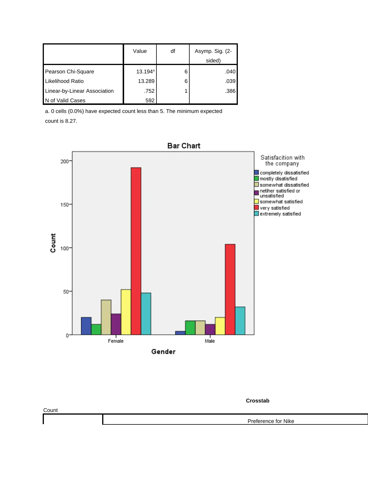
Pearson Chi-Square 13.194a 6 .040
Likelihood Ratio 13.289 6 .039
Linear-by-Linear Association .752 1 .386
N of Valid Cases 592
a. 0 cells (0.0%) have expected count less than 5. The minimum expected
count is 8.27.
Crosstab
Count
Preference for Nike
sided)
Pearson Chi-Square 13.194a 6 .040
Likelihood Ratio 13.289 6 .039
Linear-by-Linear Association .752 1 .386
N of Valid Cases 592
a. 0 cells (0.0%) have expected count less than 5. The minimum expected
count is 8.27.
Crosstab
Count
Preference for Nike
no preference at
all
very slight
preference
some preference neither have a
preference for or
not
moderate
preference
fair prefe
Gender Female 124 16 100 28 60
Male 8 24 36 36 56
Total 132 40 136 64 116
Chi-Square Tests
Value df Asymp. Sig. (2-
sided)
Pearson Chi-Square 89.125a 6 .000
Likelihood Ratio 101.503 6 .000
Linear-by-Linear Association 42.541 1 .000
N of Valid Cases 592
a. 0 cells (0.0%) have expected count less than 5. The minimum expected
count is 5.51.
Crosstab
Count
Purchase Intention for Nike
extremely unlikely unlikely somewhat unlikely netiher likely or
unlikely
likely very likely extrem
Gender Female 12 40 44 48 120 72
Male 4 28 48 32 32 32
Total 16 68 92 80 152 104
Chi-Square Tests
Count
Purchase Intention for Nike
extremely unlikely unlikely somewhat unlikely netiher likely or
unlikely
likely very likely extrem
Gender Female 12 40 44 48 120 72
Male 4 28 48 32 32 32
Total 16 68 92 80 152 104
Chi-Square Tests
Secure Best Marks with AI Grader
Need help grading? Try our AI Grader for instant feedback on your assignments.
Value df Asymp. Sig. (2-
sided)
Pearson Chi-Square 28.994a 6 .000
Likelihood Ratio 29.146 6 .000
Linear-by-Linear Association 8.171 1 .004
N of Valid Cases 588
a. 0 cells (0.0%) have expected count less than 5. The minimum expected
count is 5.44.
Crosstab
Count
Loyalty for Nike
sided)
Pearson Chi-Square 28.994a 6 .000
Likelihood Ratio 29.146 6 .000
Linear-by-Linear Association 8.171 1 .004
N of Valid Cases 588
a. 0 cells (0.0%) have expected count less than 5. The minimum expected
count is 5.44.
Crosstab
Count
Loyalty for Nike
disagree somewhat
disagree
neither disagree
or agree
somewhat agree agree strongly agree
Gender Female 164 76 36 48 52 12
Male 0 16 4 144 36 4
Total 164 92 40 192 88 16
Chi-Square Tests
Value df Asymp. Sig. (2-
sided)
Pearson Chi-Square 250.665a 5 .000
Likelihood Ratio 298.517 5 .000
Linear-by-Linear Association 140.153 1 .000
N of Valid Cases 592
a. 0 cells (0.0%) have expected count less than 5. The minimum expected count
is 5.51.
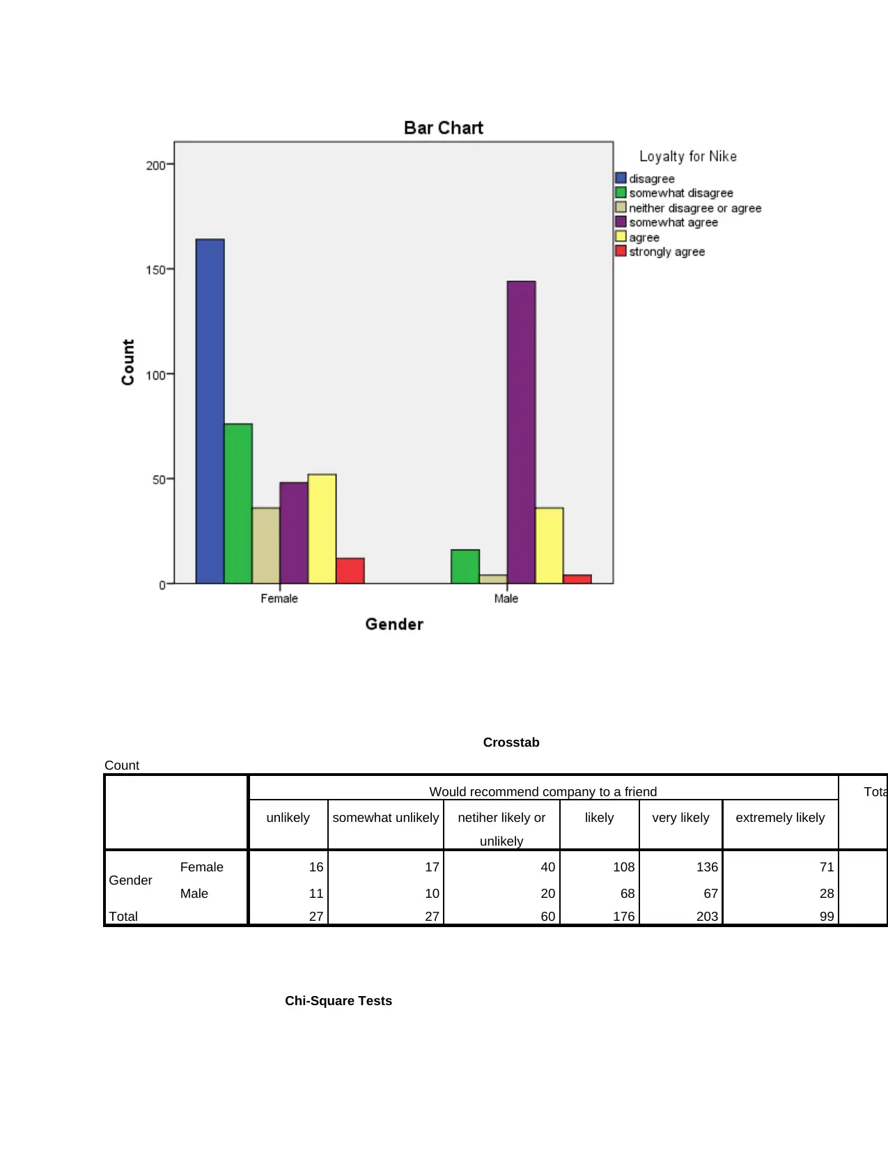
Crosstab
Count
Would recommend company to a friend Tota
unlikely somewhat unlikely netiher likely or
unlikely
likely very likely extremely likely
Gender Female 16 17 40 108 136 71
Male 11 10 20 68 67 28
Total 27 27 60 176 203 99
Chi-Square Tests
Count
Would recommend company to a friend Tota
unlikely somewhat unlikely netiher likely or
unlikely
likely very likely extremely likely
Gender Female 16 17 40 108 136 71
Male 11 10 20 68 67 28
Total 27 27 60 176 203 99
Chi-Square Tests
Paraphrase This Document
Need a fresh take? Get an instant paraphrase of this document with our AI Paraphraser
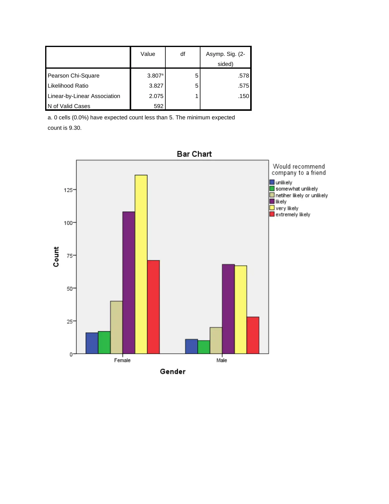
Value df Asymp. Sig. (2-
sided)
Pearson Chi-Square 3.807a 5 .578
Likelihood Ratio 3.827 5 .575
Linear-by-Linear Association 2.075 1 .150
N of Valid Cases 592
a. 0 cells (0.0%) have expected count less than 5. The minimum expected
count is 9.30.
sided)
Pearson Chi-Square 3.807a 5 .578
Likelihood Ratio 3.827 5 .575
Linear-by-Linear Association 2.075 1 .150
N of Valid Cases 592
a. 0 cells (0.0%) have expected count less than 5. The minimum expected
count is 9.30.
1 out of 26
Related Documents


Your All-in-One AI-Powered Toolkit for Academic Success.
+13062052269
info@desklib.com
Available 24*7 on WhatsApp / Email
![[object Object]](/_next/static/media/star-bottom.7253800d.svg)
Unlock your academic potential
© 2024 | Zucol Services PVT LTD | All rights reserved.