Analyzing Household Data for Statistics in Business and Finance

This article discusses the analysis of household data for Statistics in Business and Finance. It covers topics such as sampling techniques, descriptive statistics, probability distributions, and contingency tables.

Statistics For Business and Finance (BUS5SBF)
Analyzing Household Data
[Pick the date]
Student Name

Task 1
Part A
In relation to the given task, a sample of 200 observations has been taken or selected from the
given population data. This has been done using the simple random sampling whereby each of
the observation present in the population has equal chance of being selected and hence occupy a
position in the sample. Without a doubt, the simple random sampling is better than any of the
non-probability sampling methods, but a key concern with this sampling technique is that it is
quite possible that the sample may not be representative especially if the sample size is small
(Eriksson & Kovalainen, 2015). Hence an alternative sampling technique i.e. stratified random
sampling is recommended for this task. The key advantage with this sampling technique is that it
would allow that key population attributes are represented in the sample in the same proportion
as the population. This is because this sampling technique involves that the population be
segregated according to the key attributes before the samples being selected from these groups
(Hair et. al., 2015). As a result, even though it results in more representative sample but the same
is achieved at higher cost and time consumption (Flick, 2015).
Part B
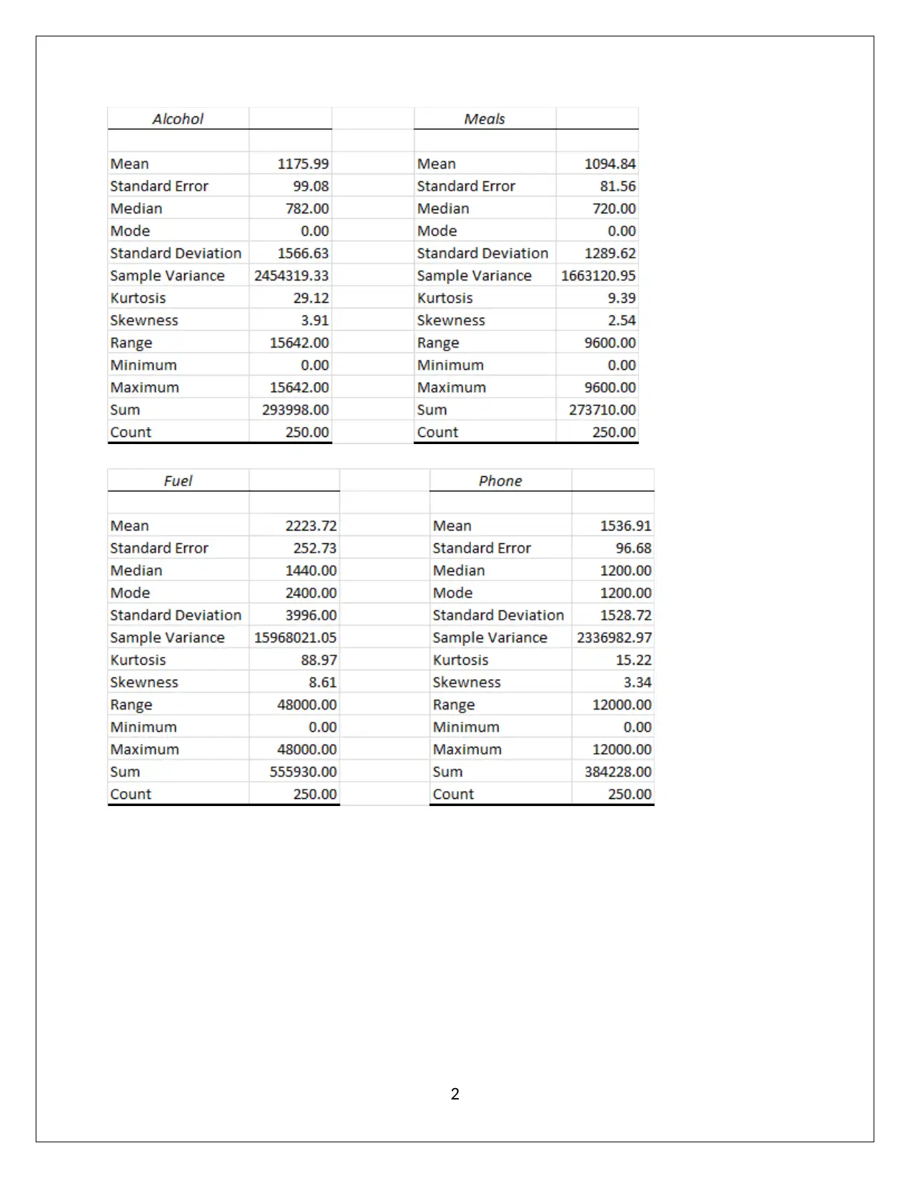
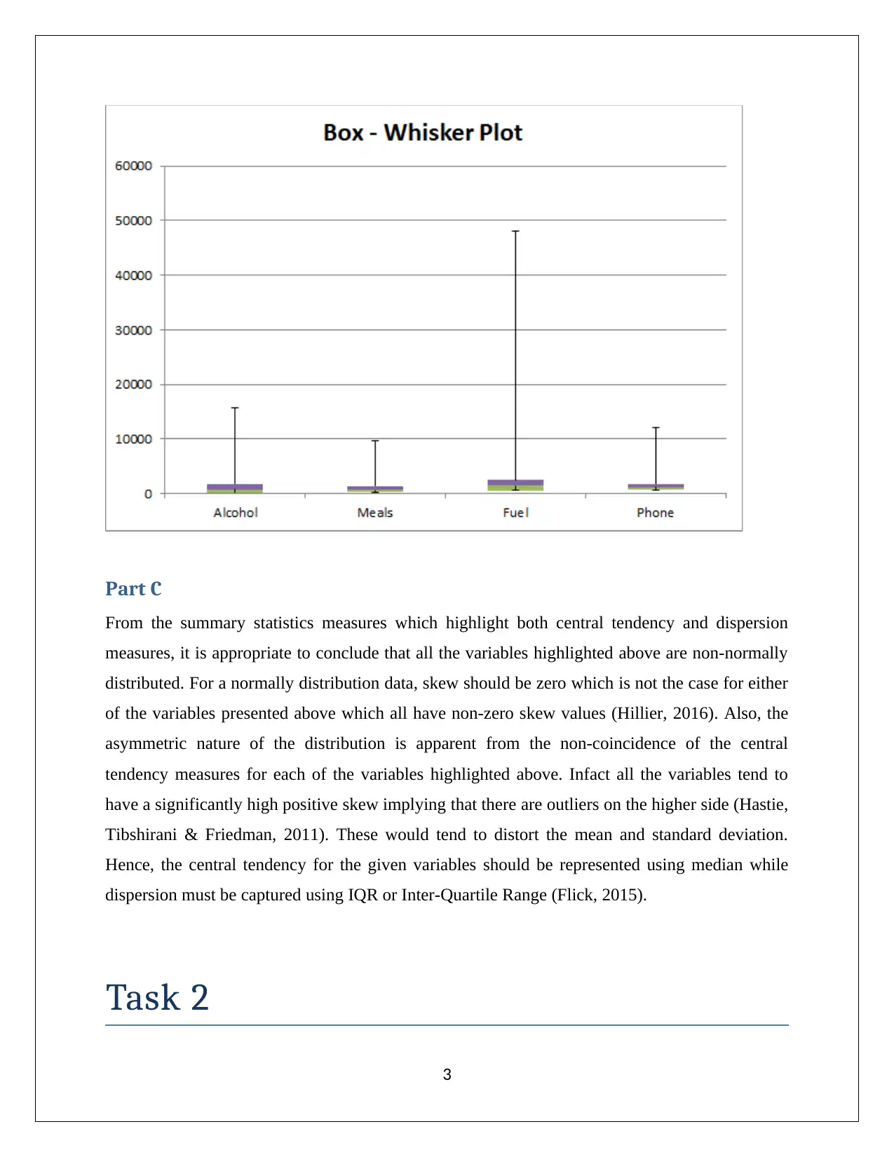
Descriptive statistics and box-whisker plot of the given variables is highlighted below:
1

2

Part C
From the summary statistics measures which highlight both central tendency and dispersion
measures, it is appropriate to conclude that all the variables highlighted above are non-normally
distributed. For a normally distribution data, skew should be zero which is not the case for either
of the variables presented above which all have non-zero skew values (Hillier, 2016). Also, the
asymmetric nature of the distribution is apparent from the non-coincidence of the central
tendency measures for each of the variables highlighted above. Infact all the variables tend to
have a significantly high positive skew implying that there are outliers on the higher side (Hastie,
Tibshirani & Friedman, 2011). These would tend to distort the mean and standard deviation.
Hence, the central tendency for the given variables should be represented using median while
dispersion must be captured using IQR or Inter-Quartile Range (Flick, 2015).
Task 2
3

Part A
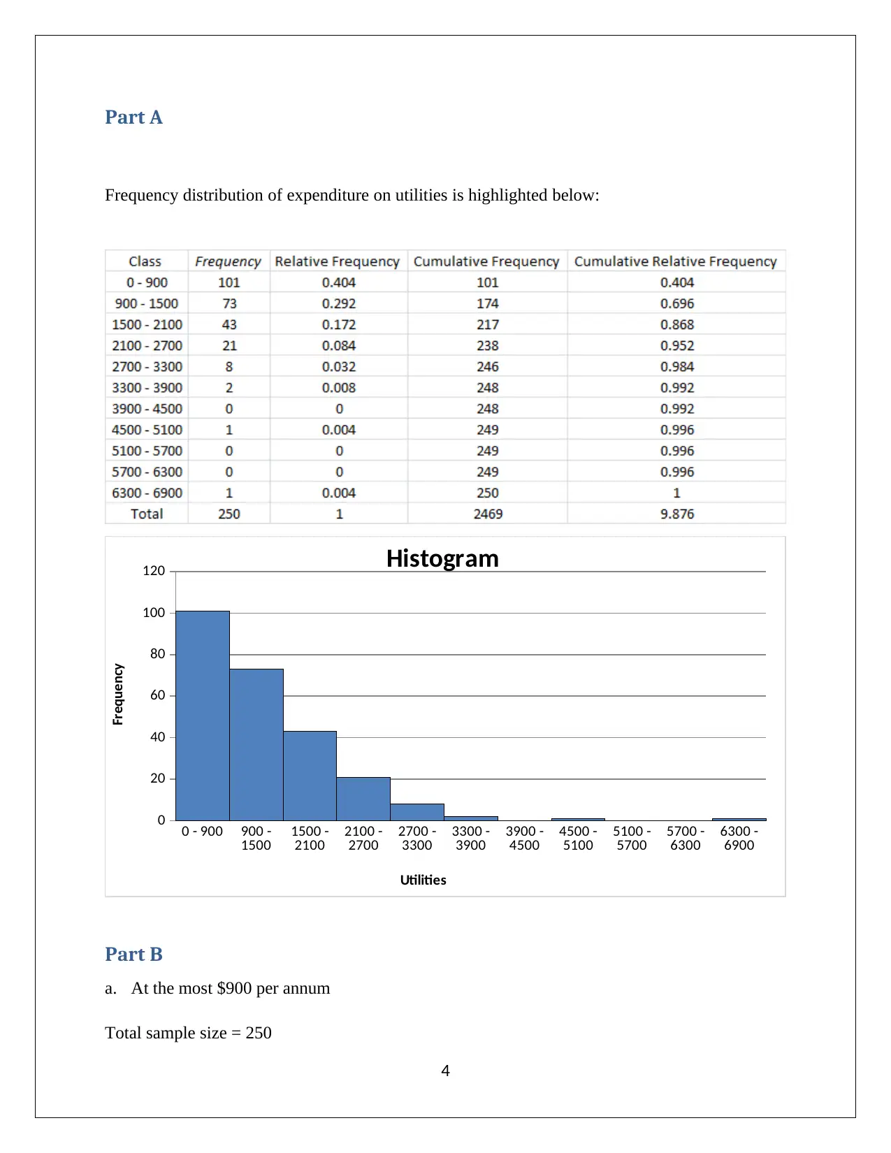
Frequency distribution of expenditure on utilities is highlighted below:
0 - 900 900 -
1500 1500 -
2100 2100 -
2700 2700 -
3300 3300 -
3900 3900 -
4500 4500 -
5100 5100 -
5700 5700 -
6300 6300 -
6900
0
20
40
60
80
100
120 Histogram
Utilities
Frequency
Part B
a. At the most $900 per annum
Total sample size = 250
4

Number of total households that have spent on utilities not greater than $900 per annum = 101
Percentage of households ¿ 101
250 =0.404
Hence, 40.4% of households have spent on utilities not greater than $900 per annum.
b. Between $1500 and $2700 per annum
Total sample size = 250
Number of total households that have spent on utilities between $1500 and $2700 per annum
=43+21
Percentage of households ¿ 64
250 =0.256
Hence, 25.6% of the households have spent on utilities between $1500 and $2700.
c. More than $3000 per annum
Total sample size = 250
Number of total households that have spent on utilities more than $3000 per annum = 10
Percentage of households ¿ 10
250 =0.04
Hence, 4% of the households have spent on utilities more than $3000 per annum.
Task 3
5

Part A
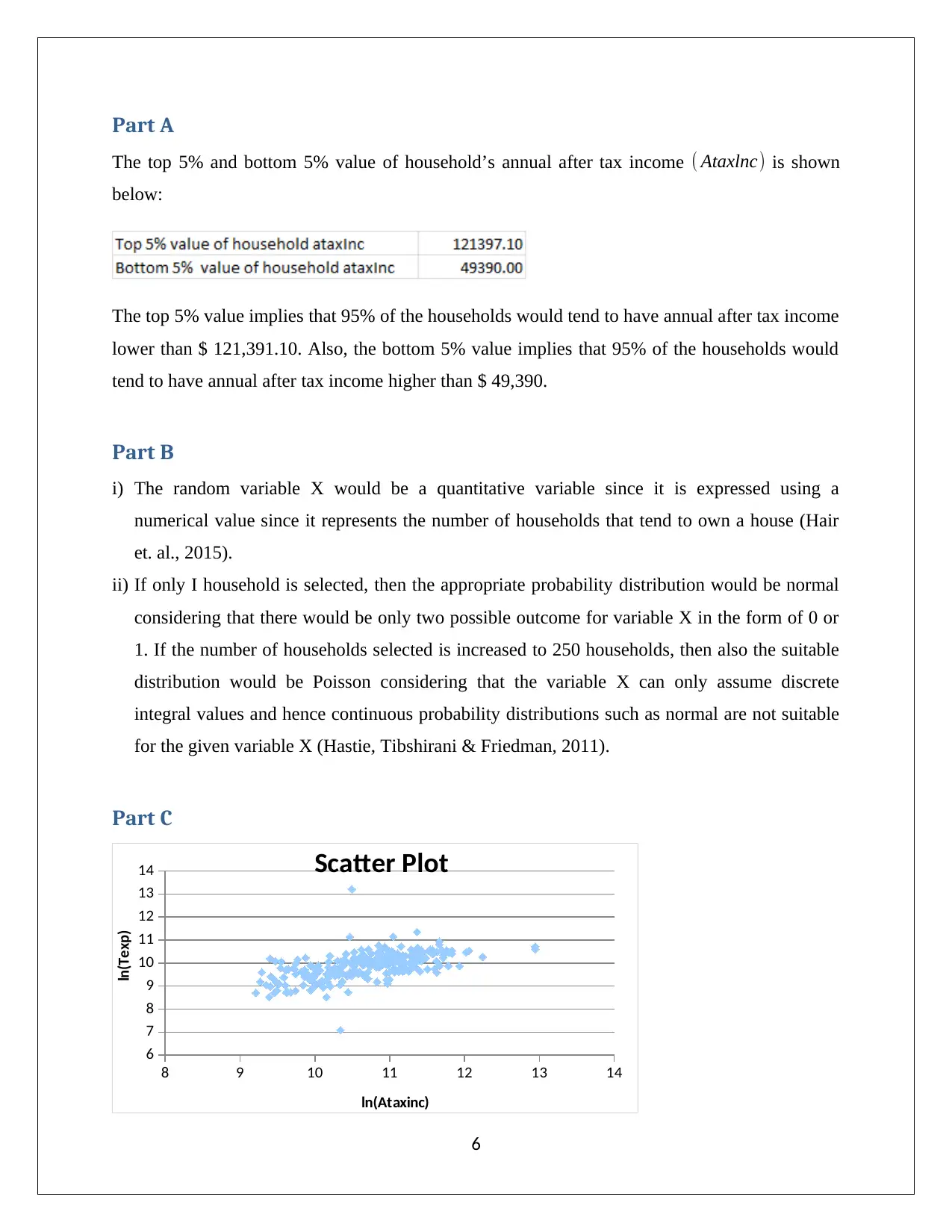
The top 5% and bottom 5% value of household’s annual after tax income ( Ataxlnc) is shown
below:
The top 5% value implies that 95% of the households would tend to have annual after tax income
lower than $ 121,391.10. Also, the bottom 5% value implies that 95% of the households would
tend to have annual after tax income higher than $ 49,390.
Part B
i) The random variable X would be a quantitative variable since it is expressed using a
numerical value since it represents the number of households that tend to own a house (Hair
et. al., 2015).
ii) If only I household is selected, then the appropriate probability distribution would be normal
considering that there would be only two possible outcome for variable X in the form of 0 or
1. If the number of households selected is increased to 250 households, then also the suitable
distribution would be Poisson considering that the variable X can only assume discrete
integral values and hence continuous probability distributions such as normal are not suitable
for the given variable X (Hastie, Tibshirani & Friedman, 2011).
Part C
8 9 10 11 12 13 14
6
7
8
9
10
11
12
13
14 Scatter Plot
ln(Ataxinc)
ln(Texp)
6

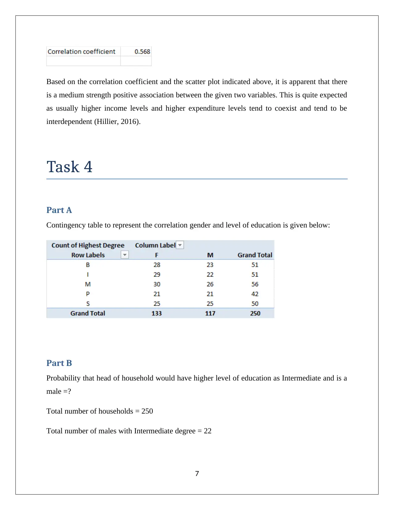
Based on the correlation coefficient and the scatter plot indicated above, it is apparent that there
is a medium strength positive association between the given two variables. This is quite expected
as usually higher income levels and higher expenditure levels tend to coexist and tend to be
interdependent (Hillier, 2016).
Task 4
Part A
Contingency table to represent the correlation gender and level of education is given below:
Part B
Probability that head of household would have higher level of education as Intermediate and is a
male =?
Total number of households = 250
Total number of males with Intermediate degree = 22
7

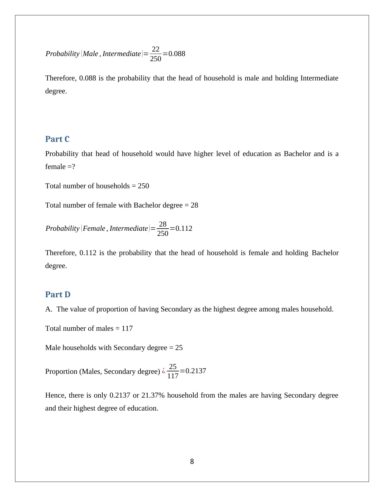
Probability ( Male , Intermediate )= 22
250 =0.088
Therefore, 0.088 is the probability that the head of household is male and holding Intermediate
degree.
Part C
Probability that head of household would have higher level of education as Bachelor and is a
female =?
Total number of households = 250
Total number of female with Bachelor degree = 28
Probability ( Female , Intermediate )= 28
250 =0.112
Therefore, 0.112 is the probability that the head of household is female and holding Bachelor
degree.
Part D
A. The value of proportion of having Secondary as the highest degree among males household.
Total number of males = 117
Male households with Secondary degree = 25
Proportion (Males, Secondary degree) ¿ 25
117 =0.2137
Hence, there is only 0.2137 or 21.37% household from the males are having Secondary degree
and their highest degree of education.
8

Part E
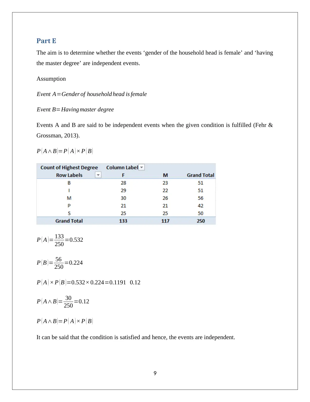
The aim is to determine whether the events ‘gender of the household head is female’ and ‘having
the master degree’ are independent events.
Assumption
Event A=Gender of household head is female
Event B=Having master degree
Events A and B are said to be independent events when the given condition is fulfilled (Fehr &
Grossman, 2013).
P ( A∧B )=P ( A ) × P ( B )
P ( A )= 133
250 =0.532
P ( B )= 56
250 =0.224
P ( A ) × P ( B )=0.532× 0.224=0.1191 0.12
P ( A∧B )= 30
250 =0.12
P ( A∧B )=P ( A ) × P ( B )
It can be said that the condition is satisfied and hence, the events are independent.
9

References
Eriksson, P. & Kovalainen, A. (2015) Quantitative methods in business research (3rd ed.).
London: Sage Publications.
Fehr, F. H., & Grossman, G. (2013) An introduction to sets, probability and hypothesis testing
(3rd ed.). Ohio: Heath.
Flick, U. (2015) Introducing research methodology: A beginner's guide to doing a research
project (4th ed.). New York: Sage Publications.
Hair, J. F., Wolfinbarger, M., Money, A. H., Samouel, P., & Page, M. J. (2015) Essentials of
business research methods (2nd ed.). New York: Routledge.
Hastie, T., Tibshirani, R. & Friedman, J. (2011) The Elements of Statistical Learning (4th
ed.). New York: Springer Publications.
Hillier, F. (2016) Introduction to Operations Research (6th ed.). New York: McGraw Hill
Publications
10