Analysis of Association between Annual Income and Online Cosmetic Expenditure

The study aims to find out if there exists an association between the annual income and the amount that is spent on cosmetics online. Additionally, the study also aims to test the hypothesis whether the gender and online cosmetic expenditure are inter-related or not. The requisite descriptive and inferential statistical techniques have been applied on the sample data. The results suggest that gender and online cosmetic spending do not show any significant relationship which suggests that no gender specific differences are observed.

STATISTICS
ASSIGNMENT
Student Name
[Pick the date]

Executive Summary
The given data has been collected using a survey and focuses on three main variables namely
gender, annual income of respondent and online cosmetic expenditure in the last 12 months. The
aim of the given study is to find out if there exists an association between the annual income and
the amount that is spent on cosmetics online. Additionally, the study also aims to test the
hypothesis whether the gender and online cosmetic expenditure are inter-related or not. In order
to analyse the same, the requisite descriptive and inferential statistical techniques have been
applied on the sample data. The association analysis involves the use of correlation and
regression analysis. On the other hand, the chi square test has been used for testing the
hypothesis regarding gender and online cosmetic spending. The results suggest that gender and
online cosmetic spending do not show any significant relationship which suggests that no gender
specific differences are observed. Also, it has been found that annual income has an impact on
the online cosmetic expenditure but the association relationship can be improved through the
addition of other prediction variables.
Research Study Description
The given research study to analyse the online spending on cosmetics by consumers in US. This
research study comes in the backdrop of rising online sales in the US. The appropriate data has
been collected through primary survey of 40 individuals across the two genders. A descriptive
research design has been used for the study whereby the focus is on testing specific hypothesis
using quantitative data that has been obtained through survey. Suitable descriptive and inferential
statistical tools would be used to analyse the given data in order to derive meaningful
conclusions. The findings and conclusion have been presented in the form of a separate section
dedicated to the same.
Hypothesis
The sample data collected would be used to test the following two hypotheses.
 Is there any significant relationship between the annual income earned by individuals and
the online spending on cosmetic?
 Does the online spending on cosmetic by an individual depend on the gender?
Variables of Interest
There are three variables which are present in the given dataset and are explained below.
1) Gender – The gender of the respondents can be male or female. Male has been denoted
with the alphabet M while Female has been denoted with the alphabet F. The data
measurement has been done using a nominal scale.
2) Annual income- This denotes the annual income of the respondents. The scale of
measurement for the given variable is interval.
1

3) Online shopping cosmetic expenditure – This refers to the amount of money that the
respondent has spent in the last one year on online shopping on cosmetics.
Descriptive Data Analysis
The objective of the descriptive statistics is to represent a representation of the given data so that
the features of the sample population can be identified. The descriptive statistics (numerical
summary) for the selected variables are highlighted below:
 Gender
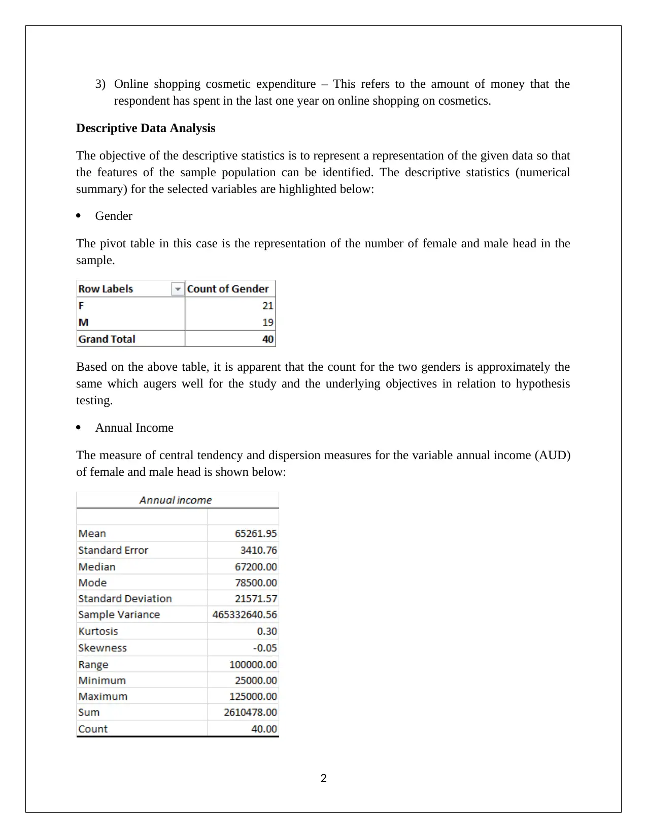
The pivot table in this case is the representation of the number of female and male head in the
sample.
Based on the above table, it is apparent that the count for the two genders is approximately the
same which augers well for the study and the underlying objectives in relation to hypothesis
testing.
 Annual Income
The measure of central tendency and dispersion measures for the variable annual income (AUD)
of female and male head is shown below:
2

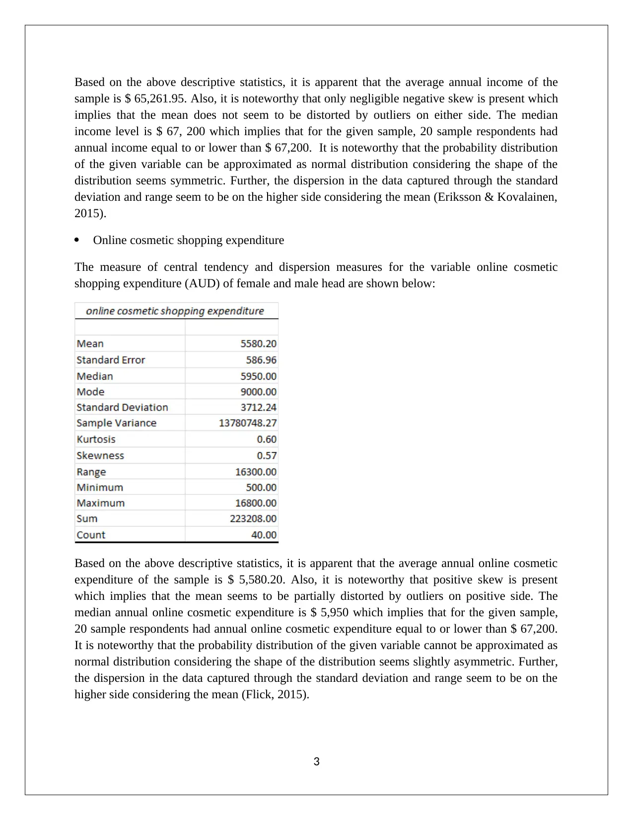
Based on the above descriptive statistics, it is apparent that the average annual income of the
sample is $ 65,261.95. Also, it is noteworthy that only negligible negative skew is present which
implies that the mean does not seem to be distorted by outliers on either side. The median
income level is $ 67, 200 which implies that for the given sample, 20 sample respondents had
annual income equal to or lower than $ 67,200. It is noteworthy that the probability distribution
of the given variable can be approximated as normal distribution considering the shape of the
distribution seems symmetric. Further, the dispersion in the data captured through the standard
deviation and range seem to be on the higher side considering the mean (Eriksson & Kovalainen,
2015).
 Online cosmetic shopping expenditure
The measure of central tendency and dispersion measures for the variable online cosmetic
shopping expenditure (AUD) of female and male head are shown below:
Based on the above descriptive statistics, it is apparent that the average annual online cosmetic
expenditure of the sample is $ 5,580.20. Also, it is noteworthy that positive skew is present
which implies that the mean seems to be partially distorted by outliers on positive side. The
median annual online cosmetic expenditure is $ 5,950 which implies that for the given sample,
20 sample respondents had annual online cosmetic expenditure equal to or lower than $ 67,200.
It is noteworthy that the probability distribution of the given variable cannot be approximated as
normal distribution considering the shape of the distribution seems slightly asymmetric. Further,
the dispersion in the data captured through the standard deviation and range seem to be on the
higher side considering the mean (Flick, 2015).
3

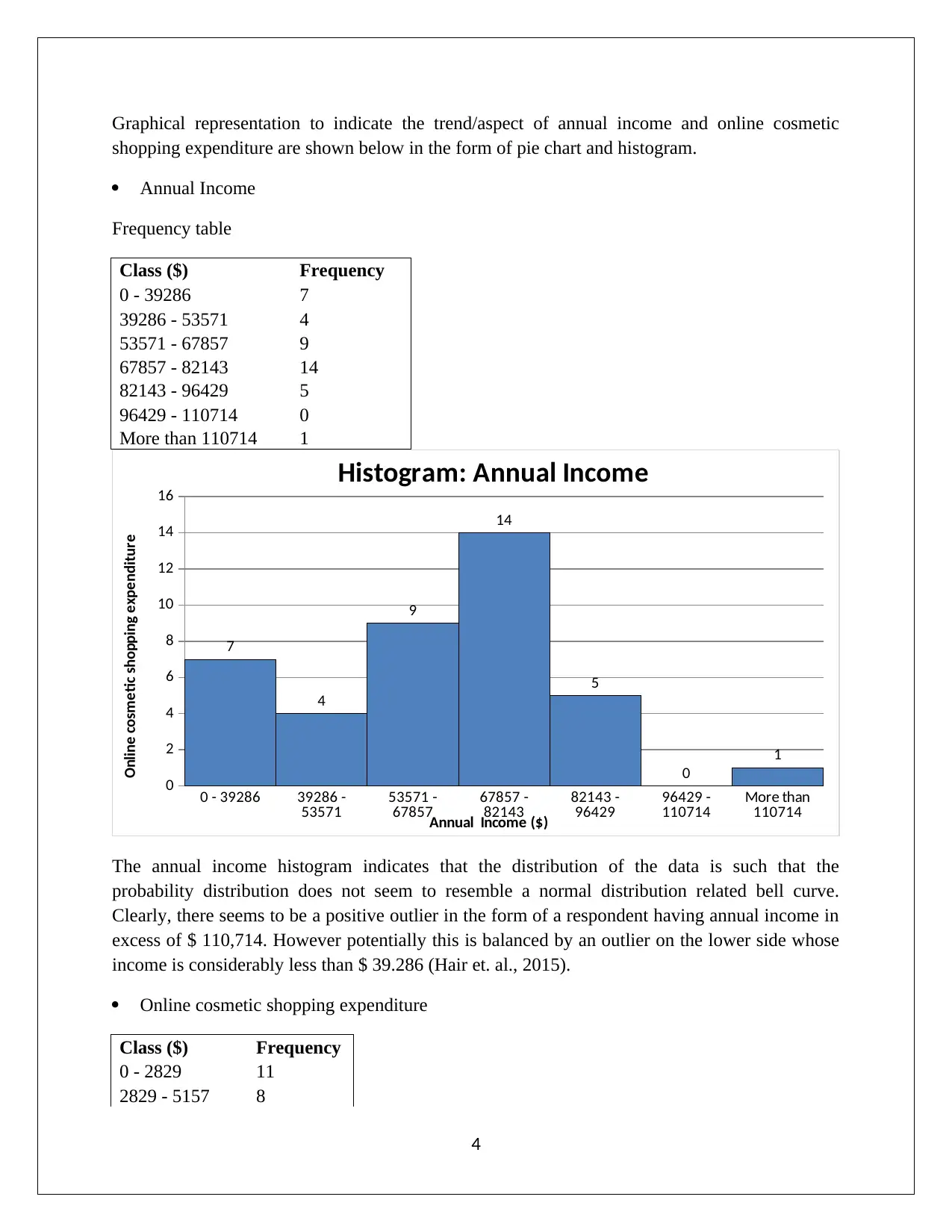
Graphical representation to indicate the trend/aspect of annual income and online cosmetic
shopping expenditure are shown below in the form of pie chart and histogram.
 Annual Income
Frequency table
Class ($) Frequency
0 - 39286 7
39286 - 53571 4
53571 - 67857 9
67857 - 82143 14
82143 - 96429 5
96429 - 110714 0
More than 110714 1
0 - 39286 39286 -
53571 53571 -
67857 67857 -
82143 82143 -
96429 96429 -
110714 More than
110714
0
2
4
6
8
10
12
14
16
7
4
9
14
5
0
1
Histogram: Annual Income
Annual Income ($)
Online cosmetic shopping expenditure
The annual income histogram indicates that the distribution of the data is such that the
probability distribution does not seem to resemble a normal distribution related bell curve.
Clearly, there seems to be a positive outlier in the form of a respondent having annual income in
excess of $ 110,714. However potentially this is balanced by an outlier on the lower side whose
income is considerably less than $ 39.286 (Hair et. al., 2015).
 Online cosmetic shopping expenditure
Class ($) Frequency
0 - 2829 11
2829 - 5157 8
4

5157 - 7486 6
7486 - 9814 12
9814 - 12143 1
12143 - 14471 1
14471 - 14471 1
0 - 2829 2829 - 5157 5157 - 7486 7486 - 9814 9814 -
12143 12143 -
14471 14471 -
14471
0
2
4
6
8
10
12
14
11
8
6
12
1 1 1
Histogram: Online cosmetic shopping
expenditure
Online cosmetic shopping expenditure ($)
Frequency
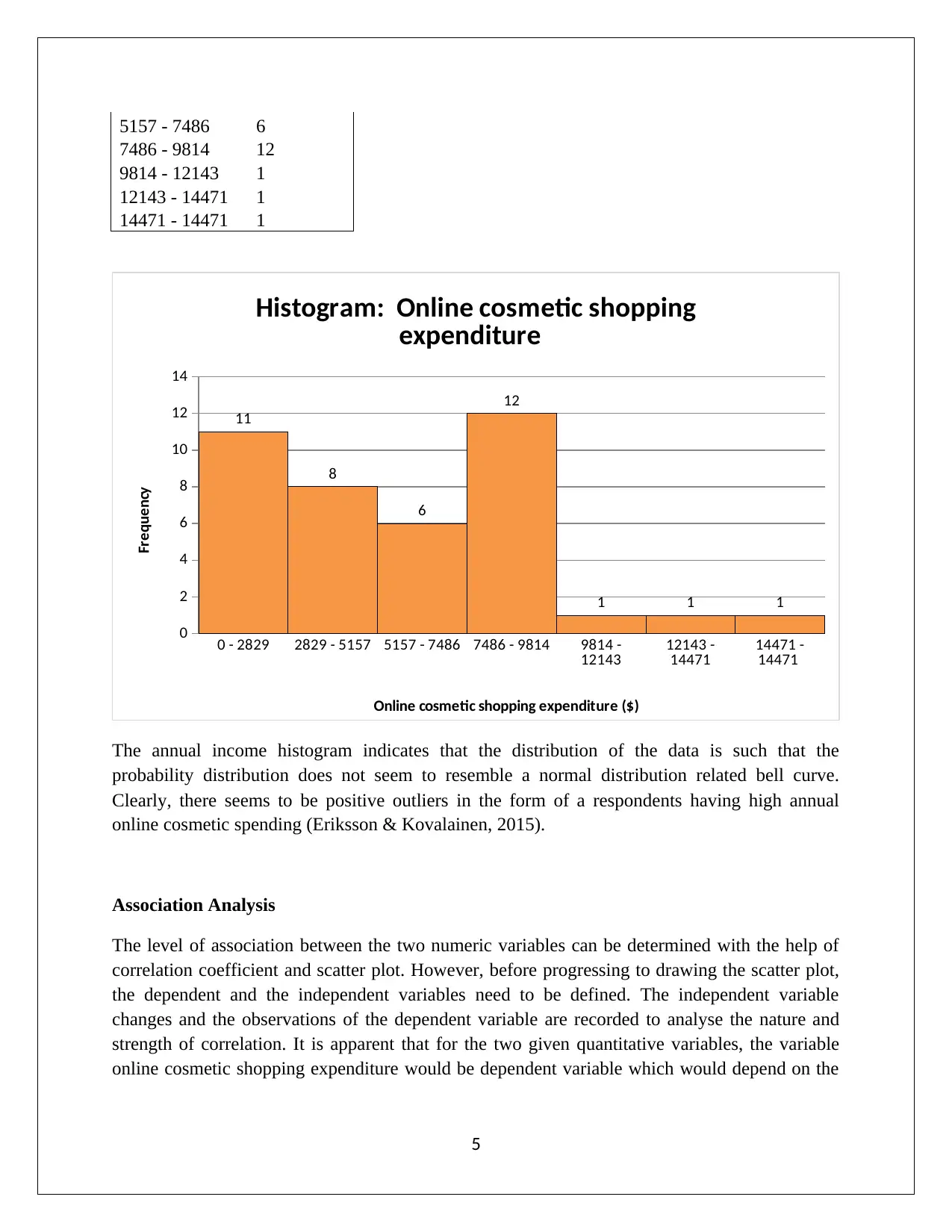
The annual income histogram indicates that the distribution of the data is such that the
probability distribution does not seem to resemble a normal distribution related bell curve.
Clearly, there seems to be positive outliers in the form of a respondents having high annual
online cosmetic spending (Eriksson & Kovalainen, 2015).
Association Analysis
The level of association between the two numeric variables can be determined with the help of
correlation coefficient and scatter plot. However, before progressing to drawing the scatter plot,
the dependent and the independent variables need to be defined. The independent variable
changes and the observations of the dependent variable are recorded to analyse the nature and
strength of correlation. It is apparent that for the two given quantitative variables, the variable
online cosmetic shopping expenditure would be dependent variable which would depend on the
5

annual income of the individual. Hence, annual income would be independent variable (Hastie,
Tibshirani & Friedman, 2011).
Hence,
x=Dependent variable
y=Independent variable
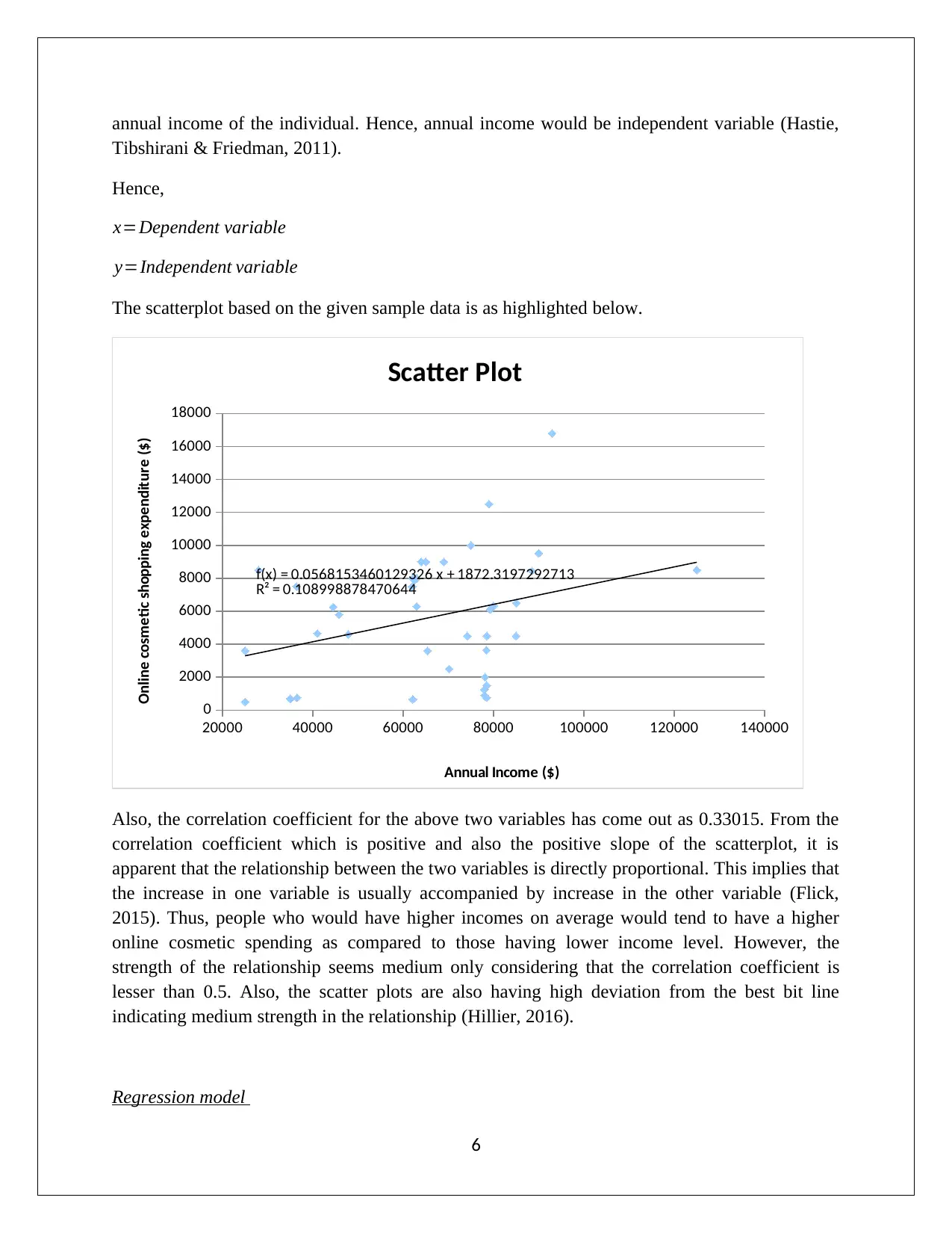
The scatterplot based on the given sample data is as highlighted below.
20000 40000 60000 80000 100000 120000 140000
0
2000
4000
6000
8000
10000
12000
14000
16000
18000
f(x) = 0.0568153460129326 x + 1872.3197292713
R² = 0.108998878470644
Scatter Plot
Annual Income ($)
Online cosmetic shopping expenditure ($)
Also, the correlation coefficient for the above two variables has come out as 0.33015. From the
correlation coefficient which is positive and also the positive slope of the scatterplot, it is
apparent that the relationship between the two variables is directly proportional. This implies that
the increase in one variable is usually accompanied by increase in the other variable (Flick,
2015). Thus, people who would have higher incomes on average would tend to have a higher
online cosmetic spending as compared to those having lower income level. However, the
strength of the relationship seems medium only considering that the correlation coefficient is
lesser than 0.5. Also, the scatter plots are also having high deviation from the best bit line
indicating medium strength in the relationship (Hillier, 2016).
Regression model
6

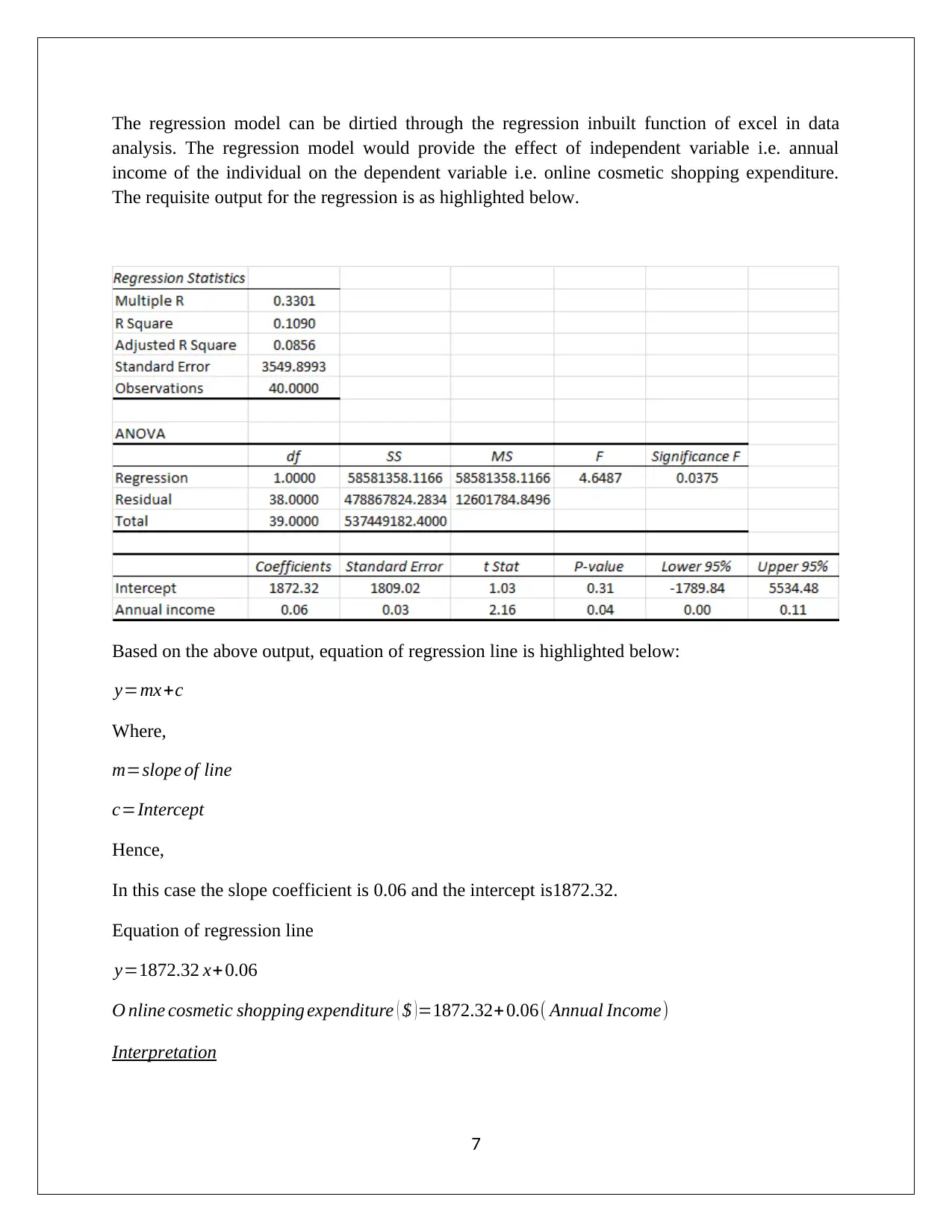
The regression model can be dirtied through the regression inbuilt function of excel in data
analysis. The regression model would provide the effect of independent variable i.e. annual
income of the individual on the dependent variable i.e. online cosmetic shopping expenditure.
The requisite output for the regression is as highlighted below.
Based on the above output, equation of regression line is highlighted below:
y=mx+c
Where,
m=slope of line
c=Intercept
Hence,
In this case the slope coefficient is 0.06 and the intercept is1872.32.
Equation of regression line
y=1872.32 x+ 0.06
O nline cosmetic shopping expenditure ( $ ) =1872.32+ 0.06( Annual Income)
Interpretation
7

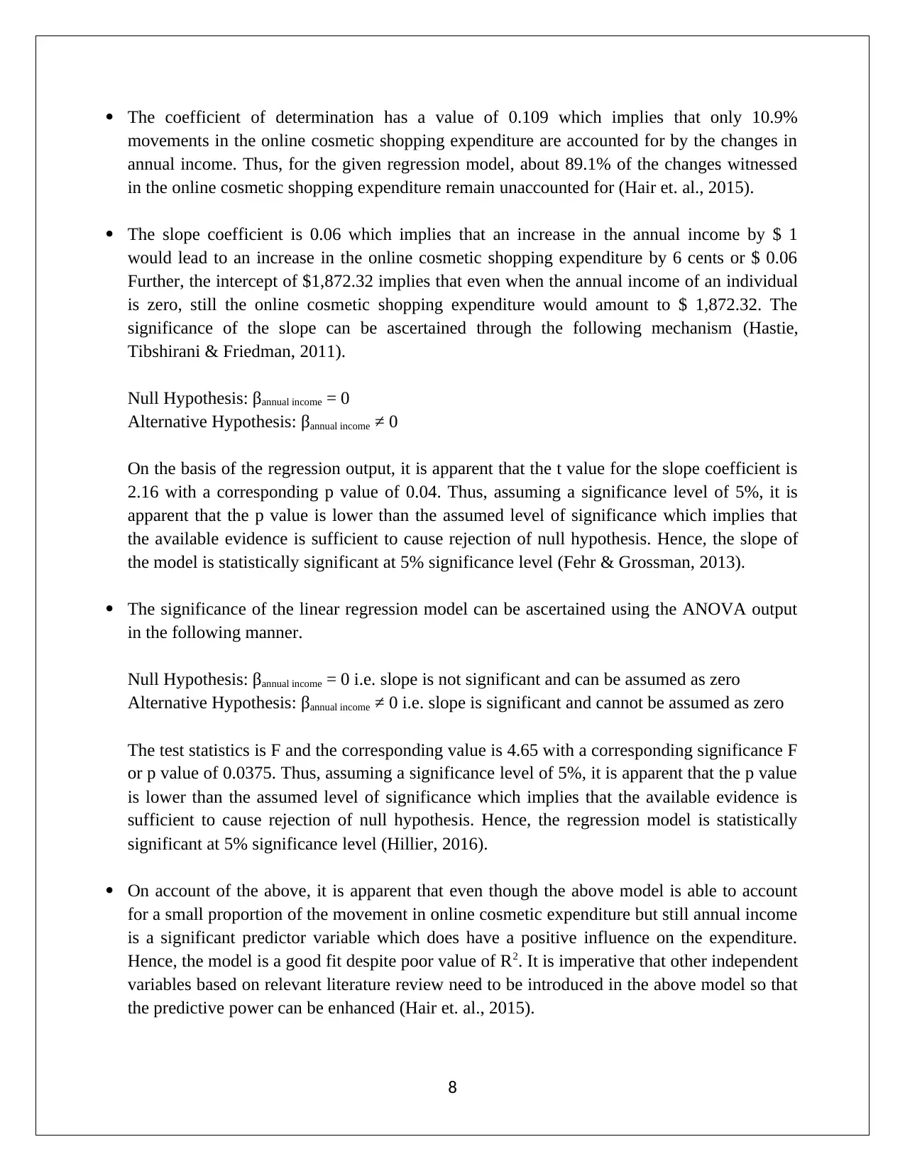
 The coefficient of determination has a value of 0.109 which implies that only 10.9%
movements in the online cosmetic shopping expenditure are accounted for by the changes in
annual income. Thus, for the given regression model, about 89.1% of the changes witnessed
in the online cosmetic shopping expenditure remain unaccounted for (Hair et. al., 2015).
 The slope coefficient is 0.06 which implies that an increase in the annual income by $ 1
would lead to an increase in the online cosmetic shopping expenditure by 6 cents or $ 0.06
Further, the intercept of $1,872.32 implies that even when the annual income of an individual
is zero, still the online cosmetic shopping expenditure would amount to $ 1,872.32. The
significance of the slope can be ascertained through the following mechanism (Hastie,
Tibshirani & Friedman, 2011).
Null Hypothesis: βannual income = 0
Alternative Hypothesis: βannual income ≠ 0
On the basis of the regression output, it is apparent that the t value for the slope coefficient is
2.16 with a corresponding p value of 0.04. Thus, assuming a significance level of 5%, it is
apparent that the p value is lower than the assumed level of significance which implies that
the available evidence is sufficient to cause rejection of null hypothesis. Hence, the slope of
the model is statistically significant at 5% significance level (Fehr & Grossman, 2013).
 The significance of the linear regression model can be ascertained using the ANOVA output
in the following manner.
Null Hypothesis: βannual income = 0 i.e. slope is not significant and can be assumed as zero
Alternative Hypothesis: βannual income ≠ 0 i.e. slope is significant and cannot be assumed as zero
The test statistics is F and the corresponding value is 4.65 with a corresponding significance F
or p value of 0.0375. Thus, assuming a significance level of 5%, it is apparent that the p value
is lower than the assumed level of significance which implies that the available evidence is
sufficient to cause rejection of null hypothesis. Hence, the regression model is statistically
significant at 5% significance level (Hillier, 2016).
 On account of the above, it is apparent that even though the above model is able to account
for a small proportion of the movement in online cosmetic expenditure but still annual income
is a significant predictor variable which does have a positive influence on the expenditure.
Hence, the model is a good fit despite poor value of R2. It is imperative that other independent
variables based on relevant literature review need to be introduced in the above model so that
the predictive power can be enhanced (Hair et. al., 2015).
8

Hypothesis Testing
The hypothesis testing is an inferential technique whereby the claim is usually captured using
hypothesis and then testing is performed to find out if the null hypothesis can be rejected or not
at the given significance level. It is a technique to derive the characteristics of the population
based on the given sample data. The objective of this hypothesis testing is to test the hypothesis
is any statistically significant relationship does exist between gender and online cosmetic
spending (Flick, 2015). It is noteworthy that gender is a nominal variable whereas online
spending on cosmetics is a numerical or quantitative variable. The potential interdependence
between these two variables can be tested using the Chi –Square test. However, in order to
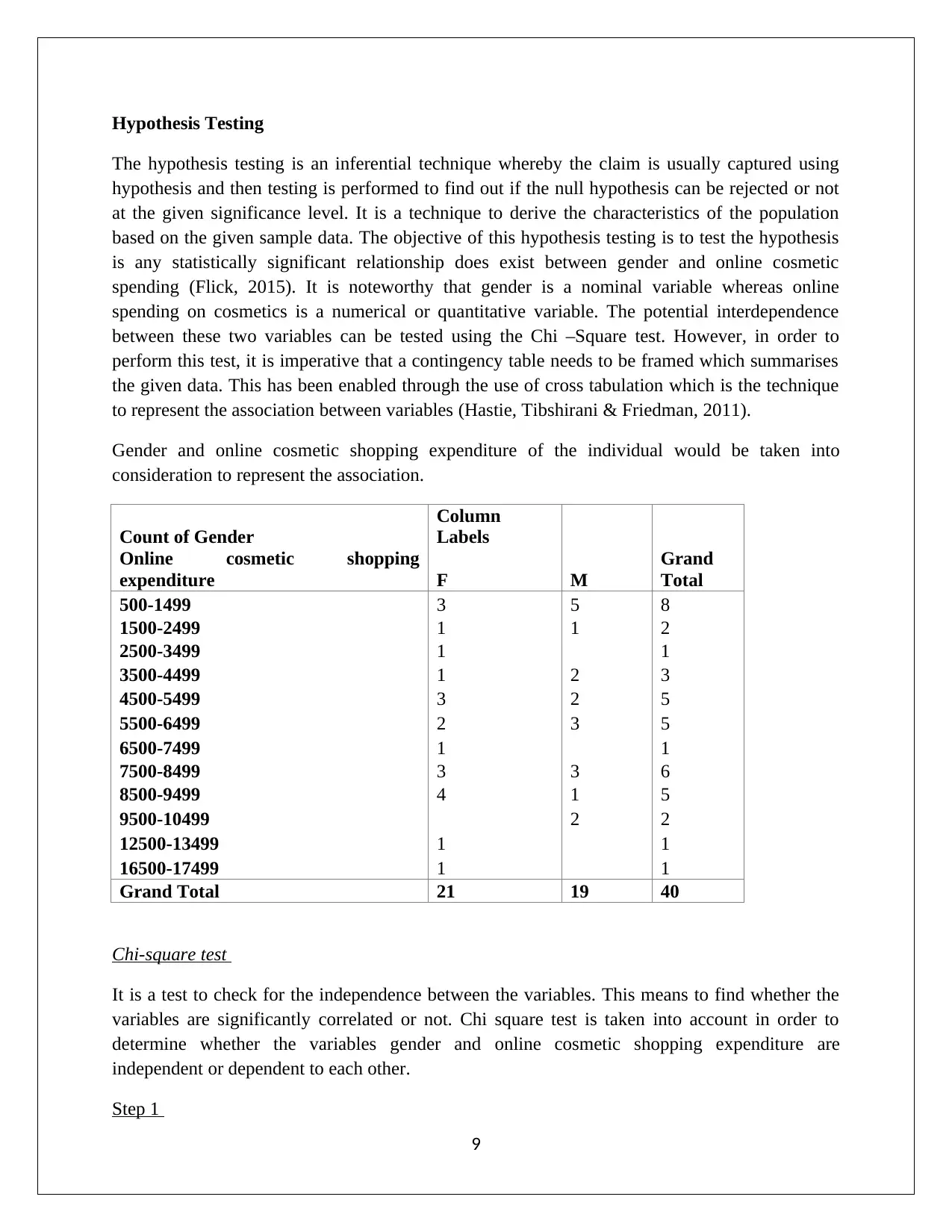
perform this test, it is imperative that a contingency table needs to be framed which summarises
the given data. This has been enabled through the use of cross tabulation which is the technique
to represent the association between variables (Hastie, Tibshirani & Friedman, 2011).
Gender and online cosmetic shopping expenditure of the individual would be taken into
consideration to represent the association.
Count of Gender
Column
Labels
Online cosmetic shopping
expenditure F M
Grand
Total
500-1499 3 5 8
1500-2499 1 1 2
2500-3499 1 1
3500-4499 1 2 3
4500-5499 3 2 5
5500-6499 2 3 5
6500-7499 1 1
7500-8499 3 3 6
8500-9499 4 1 5
9500-10499 2 2
12500-13499 1 1
16500-17499 1 1
Grand Total 21 19 40
Chi-square test
It is a test to check for the independence between the variables. This means to find whether the
variables are significantly correlated or not. Chi square test is taken into account in order to
determine whether the variables gender and online cosmetic shopping expenditure are
independent or dependent to each other.
Step 1
9

The requisite hypotheses or the given statistical test are shown below:
Null hypothesis H0 :Gender and online cosmetic shopping expenditure are independent variables.
Alternative hypothesis H1 :Gender and online cosmetic shopping expenditure are dependent
variables.
Step 2
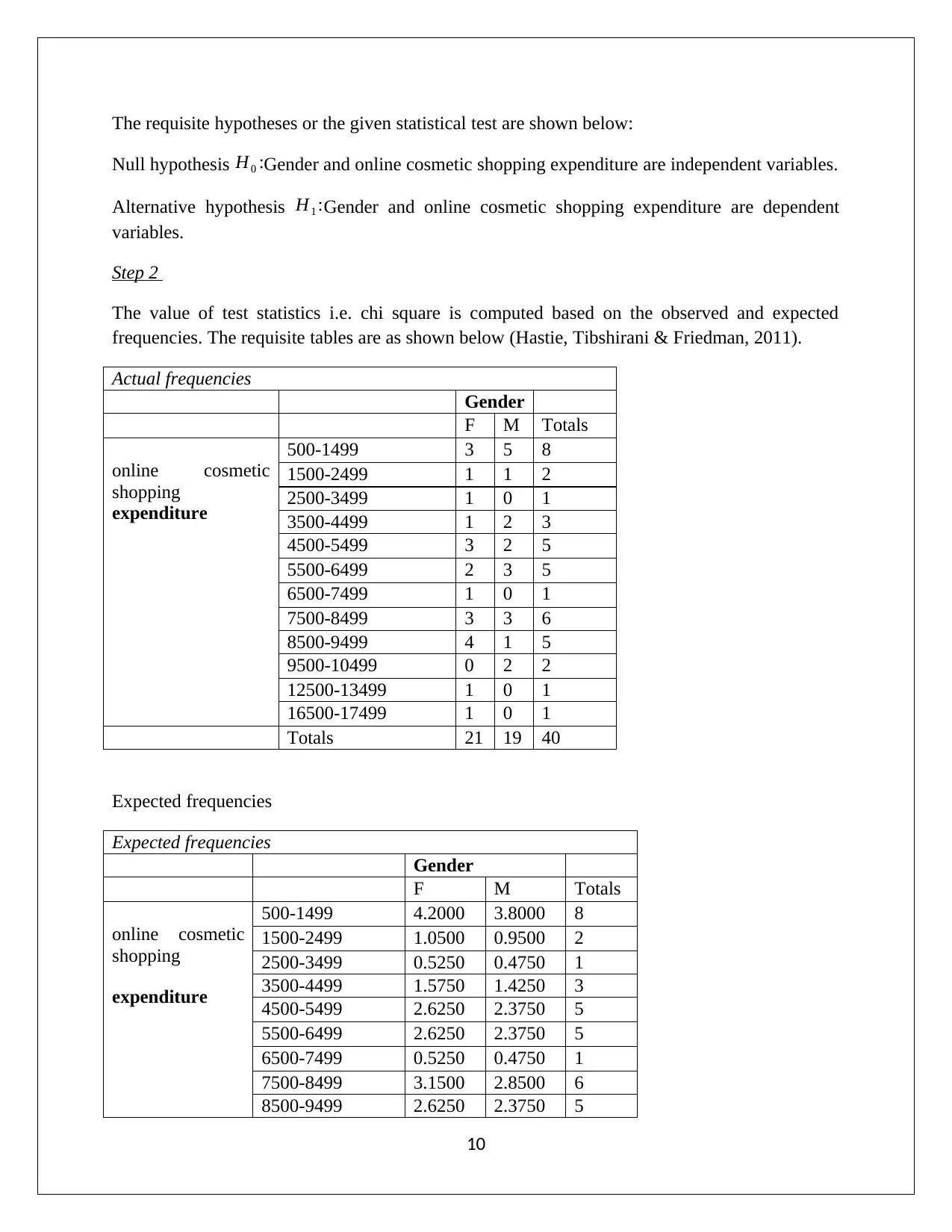
The value of test statistics i.e. chi square is computed based on the observed and expected
frequencies. The requisite tables are as shown below (Hastie, Tibshirani & Friedman, 2011).
Actual frequencies
Gender
F M Totals
online cosmetic
shopping
expenditure
500-1499 3 5 8
1500-2499 1 1 2
2500-3499 1 0 1
3500-4499 1 2 3
4500-5499 3 2 5
5500-6499 2 3 5
6500-7499 1 0 1
7500-8499 3 3 6
8500-9499 4 1 5
9500-10499 0 2 2
12500-13499 1 0 1
16500-17499 1 0 1
Totals 21 19 40
Expected frequencies
Expected frequencies
Gender
F M Totals
online cosmetic
shopping
expenditure
500-1499 4.2000 3.8000 8
1500-2499 1.0500 0.9500 2
2500-3499 0.5250 0.4750 1
3500-4499 1.5750 1.4250 3
4500-5499 2.6250 2.3750 5
5500-6499 2.6250 2.3750 5
6500-7499 0.5250 0.4750 1
7500-8499 3.1500 2.8500 6
8500-9499 2.6250 2.3750 5
10

9500-10499 1.0500 0.9500 2
12500-13499 0.5250 0.4750 1
16500-17499 0.5250 0.4750 1
Totals 21 19 40
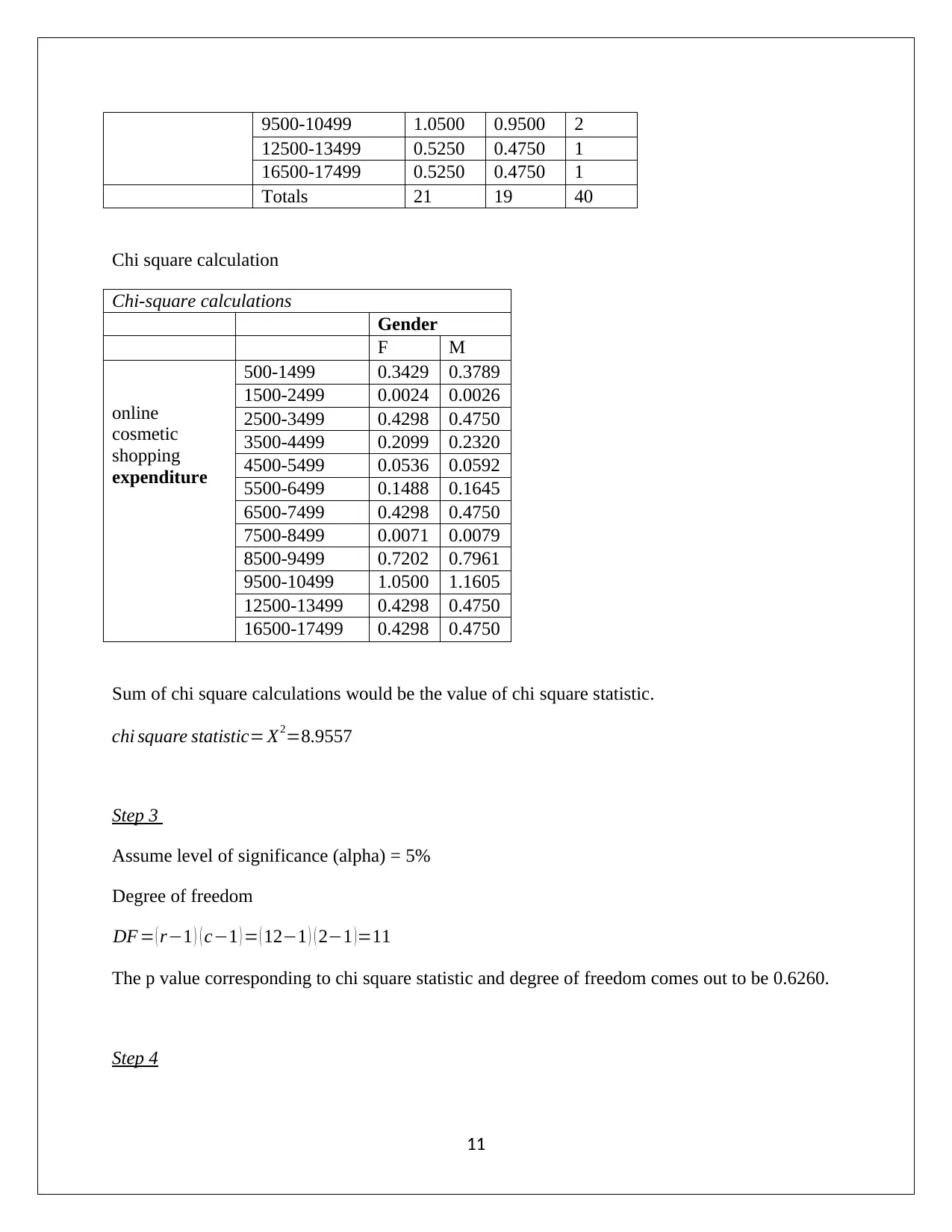
Chi square calculation
Chi-square calculations
Gender
F M
online
cosmetic
shopping
expenditure
500-1499 0.3429 0.3789
1500-2499 0.0024 0.0026
2500-3499 0.4298 0.4750
3500-4499 0.2099 0.2320
4500-5499 0.0536 0.0592
5500-6499 0.1488 0.1645
6500-7499 0.4298 0.4750
7500-8499 0.0071 0.0079
8500-9499 0.7202 0.7961
9500-10499 1.0500 1.1605
12500-13499 0.4298 0.4750
16500-17499 0.4298 0.4750
Sum of chi square calculations would be the value of chi square statistic.
chi square statistic= X2=8.9557
Step 3
Assume level of significance (alpha) = 5%
Degree of freedom
DF = ( r−1 ) ( c−1 ) = ( 12−1 ) ( 2−1 ) =11
The p value corresponding to chi square statistic and degree of freedom comes out to be 0.6260.
Step 4
11

It can be seen from the above that p value for the input chi square and degree of freedom comes
out to be 0.6260 which is higher than the assumed level of significance. Therefore, the
conclusion can be drawn that insufficient evidences is present to reject the null hypothesis and to
accept the alternative hypothesis. Hence, it can be said that variables gender and online cosmetic
shopping expenditure are independent of each other. Further, no statistically significant
association is exist between the two variables. Thus, this implies that online cosmetic shopping is
not limited by females but males also tend to match their fairer counterparts (Hair et. al, 2015).
Findings & Limitations
Based on the above analysis, it is apparent that there is a significant relationship between the
income level of individuals and the amount they tend to spend in online cosmetic shopping.
However, the relationship between these two variables is not very strong and also needs to be
assisted with other independent variables so that a better understanding and predictability of the
online cosmetic spending can be developed. Additionally, the hypothesis that gender and online
cosmetic spending are dependent is not supported by the given sample data. A chi-square test
was conducted where the conclusion drawn was that at 5% significance level, the claim
regarding dependence was rejected and hence it was indicated that no significant relationship is
found between gender and the online cosmetic spend.
A key limitation of the given study was that the sampling technique was not appropriate since
convenience sampling was used and hence bias may be present in the data. Also, only gender as
an attribute was represented (Flick, 2015). It may be possible that there are other attributes such
as race, location which can impact the spending on online cosmetic. Any further research on the
subject should focus on a higher sample size which comprises of a more representative sample
selected through the use of probability sampling technique (Hastie, Tibshirani & Friedman,
2011).
References
12

Eriksson, P. & Kovalainen, A. (2015) Quantitative methods in business research (3rd ed.).
London: Sage Publications.
Fehr, F. H., & Grossman, G. (2013) An introduction to sets, probability and hypothesis testing
(3rd ed.). Ohio: Heath.
Flick, U. (2015) Introducing research methodology: A beginner's guide to doing a research
project (4th ed.). New York: Sage Publications.
Hair, J. F., Wolfinbarger, M., Money, A. H., Samouel, P., & Page, M. J. (2015) Essentials of
business research methods (2nd ed.). New York: Routledge.
Hastie, T., Tibshirani, R. & Friedman, J. (2011) The Elements of Statistical Learning (4th
ed.). New York: Springer Publications.
Hillier, F. (2016) Introduction to Operations Research (6th ed.). New York: McGraw Hill
Publications.
Koch, K.R. (2013). Parameter Estimation and Hypothesis Testing in Linear Models (2nd ed.).
London: Springer Science & Business Media.
13