[Analysis of Employee Earnings Data]

The provided document appears to be a statistical analysis of employee earnings data, possibly from a survey or census. It contains various numerical values and statistics for different demographic categories, such as gender, age range, occupation code, and lodging method. The data is presented in a table with multiple columns, including mean, standard error, median, mode, standard deviation, sample variance, kurtosis, and skewness. This analysis may be used to understand trends and patterns in employee earnings, potentially informing policy or business decisions.

Assessment Report- Taxation

EXECUTIVE SUMMARY
To analysing the dependency of people in terms of making the taxable payment is the prime
requirement of the government. In the preset report there has been analysis of various data set on
the basis of setting the frequencies and the various observations. Further, there will be
calculations relevant with correlation and regressions techniques which will help in determining
the appropriate relationship among the selected variables.

Table of Contents
PART A...........................................................................................................................................1
1 Selection of the random sample...............................................................................................1
2 Descriptive Statistics................................................................................................................2
PART B............................................................................................................................................3
3 Confidence Intervals................................................................................................................3
4 Hypothesis Testing...................................................................................................................4
5 Correlation................................................................................................................................5
CONCLUSION................................................................................................................................6
REFERENCES................................................................................................................................7
APPENDIX......................................................................................................................................8

PART A
1 Selection of the random sample
Row Labels Count of Lodgement_method Percentage
2 33 55%
1 27 45.00%
Grand Total 60 100.00%
2 1
0
5
10
15
20
25
30
35
Count of Lodgement_method
Percentage
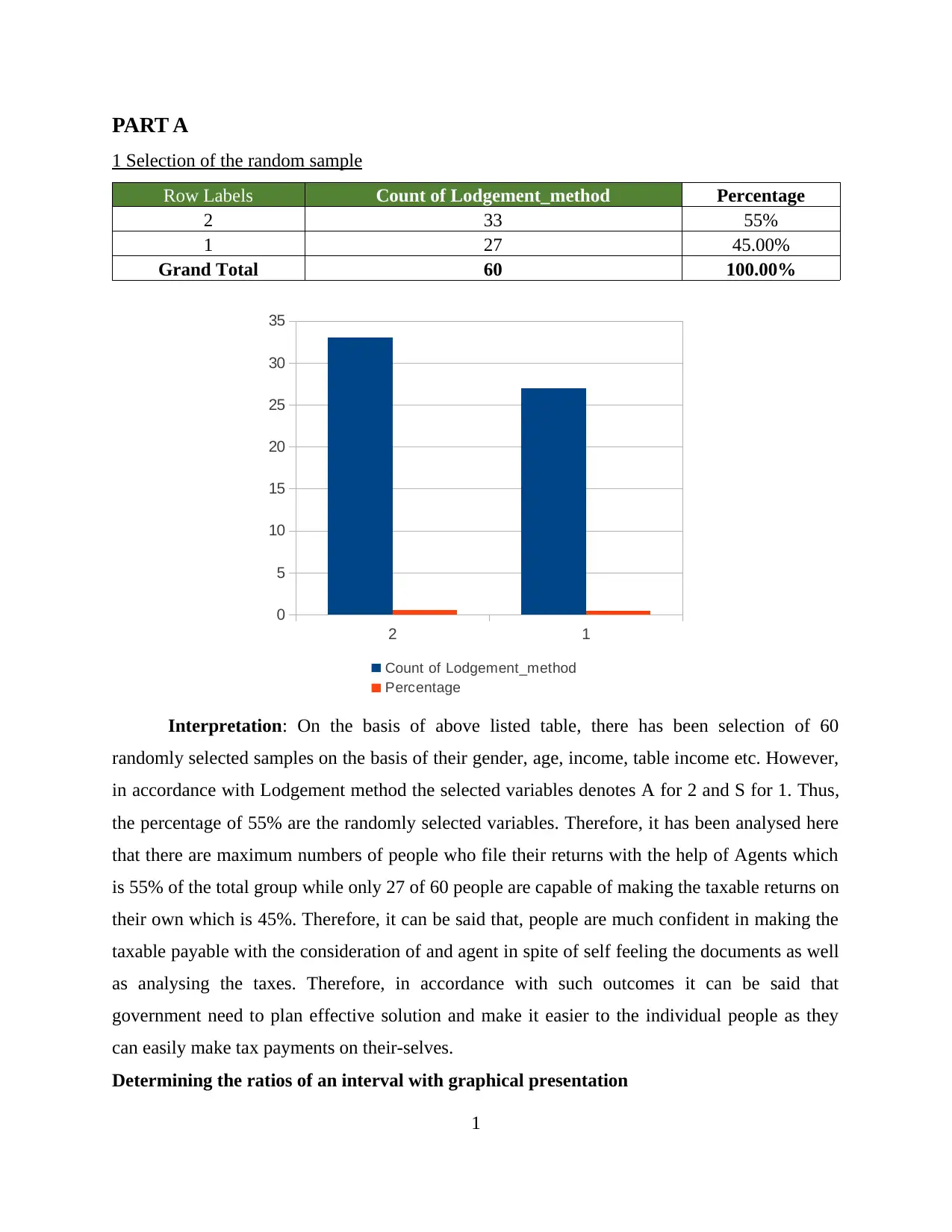
Interpretation: On the basis of above listed table, there has been selection of 60
randomly selected samples on the basis of their gender, age, income, table income etc. However,
in accordance with Lodgement method the selected variables denotes A for 2 and S for 1. Thus,
the percentage of 55% are the randomly selected variables. Therefore, it has been analysed here
that there are maximum numbers of people who file their returns with the help of Agents which
is 55% of the total group while only 27 of 60 people are capable of making the taxable returns on
their own which is 45%. Therefore, it can be said that, people are much confident in making the
taxable payable with the consideration of and agent in spite of self feeling the documents as well
as analysing the taxes. Therefore, in accordance with such outcomes it can be said that
government need to plan effective solution and make it easier to the individual people as they
can easily make tax payments on their-selves.
Determining the ratios of an interval with graphical presentation
1

Tot_inc_amt
Mean 43051.35
Standard Error 3990.25959
Median 36033.5
Mode #N/A
Standard Deviation 30908.4178
Sample Variance 955330294
Kurtosis 1.28035412
Skewness 1.26092191
Range 136798
Minimum 3246
Maximum 140044
Sum 2583081
Count 60
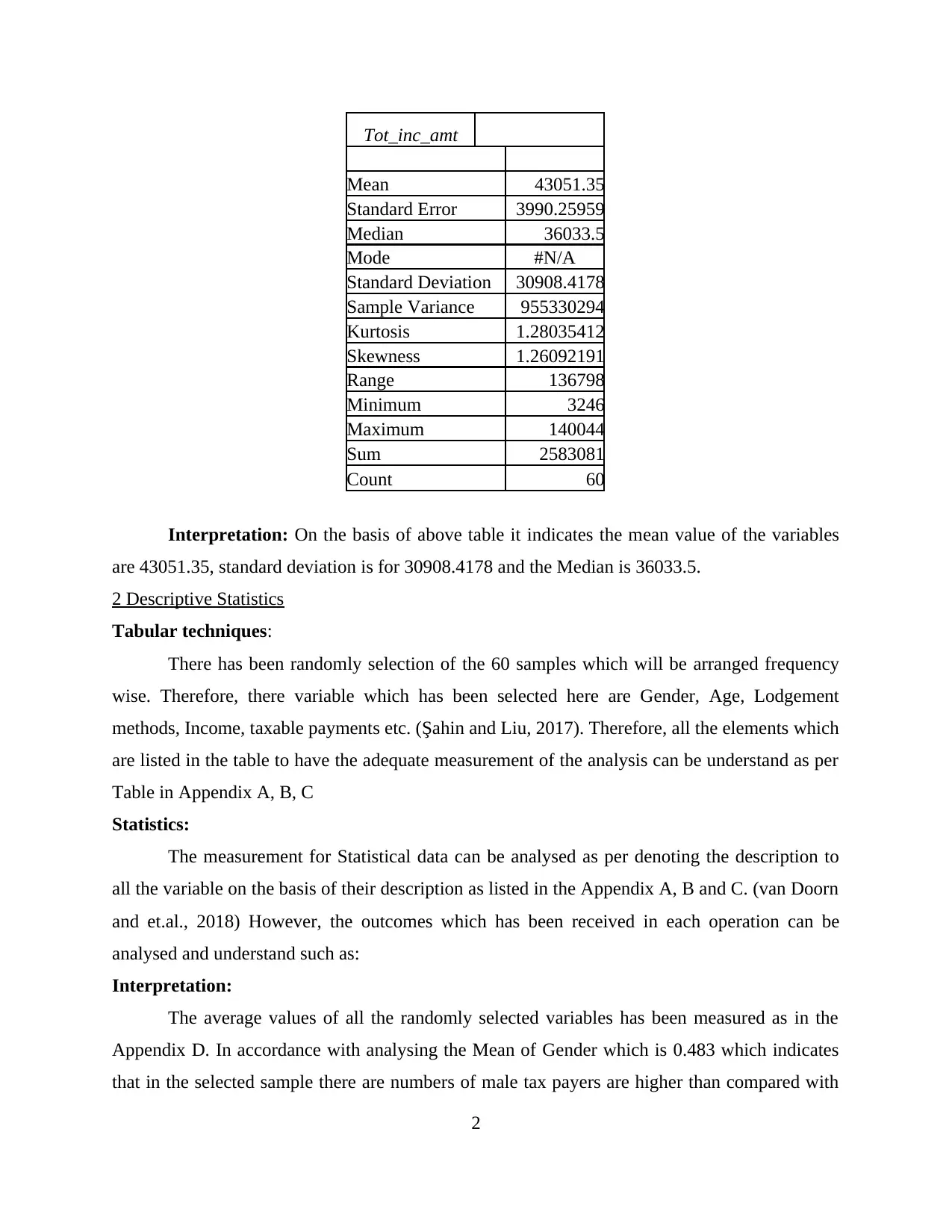
Interpretation: On the basis of above table it indicates the mean value of the variables
are 43051.35, standard deviation is for 30908.4178 and the Median is 36033.5.
2 Descriptive Statistics
Tabular techniques:
There has been randomly selection of the 60 samples which will be arranged frequency
wise. Therefore, there variable which has been selected here are Gender, Age, Lodgement
methods, Income, taxable payments etc. (Şahin and Liu, 2017). Therefore, all the elements which
are listed in the table to have the adequate measurement of the analysis can be understand as per
Table in Appendix A, B, C
Statistics:
The measurement for Statistical data can be analysed as per denoting the description to
all the variable on the basis of their description as listed in the Appendix A, B and C. (van Doorn
and et.al., 2018) However, the outcomes which has been received in each operation can be
analysed and understand such as:
Interpretation:
The average values of all the randomly selected variables has been measured as in the
Appendix D. In accordance with analysing the Mean of Gender which is 0.483 which indicates
that in the selected sample there are numbers of male tax payers are higher than compared with
2

the female. In relation with the mean value of Age range which is 4.83 it indicates that there are
maximum numbers of taxpayer of age between 49-54. Thus, while analysing the occupational
code's mean value it indicates 4.48 which presents that in the selected group there are large
numbers of employees from the community and personal service sector. In accordance with the
mean value of lodgement it determines that there are comparatively equivalent lodgement
methods such as through self efforts or through agents.
In accordance with the mode value of all the variables the Gender as 0(Male), age range
as 2 (60-64), occupational code as 0, Lodgement has 2 etc. However, it can be said that such
variables bring the knowledge that there are large numbers of male tax payers who are making
the taxable payments. Therefore, the median of such variables are gender as 0, age range as 4.5,
occupational code as 4.5, lodgement as 2 and on. However, it can be said that the selected
samples are very helpful as it determines that there are maximum numbers of male tex
practitioners and they belong to the age group between 60-64 which are working in the sector of
community and personal service sector.
PART B
3 Confidence Intervals
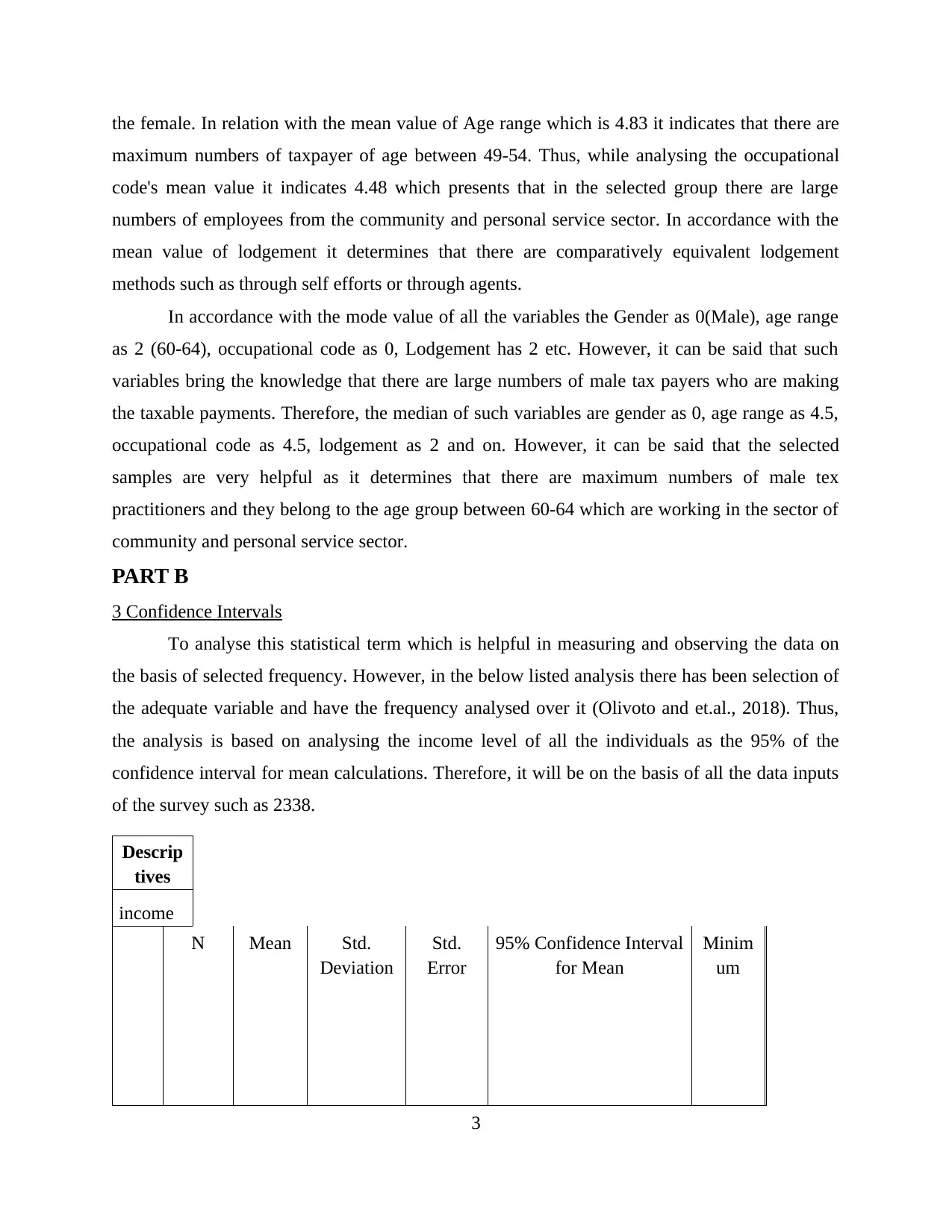
To analyse this statistical term which is helpful in measuring and observing the data on
the basis of selected frequency. However, in the below listed analysis there has been selection of
the adequate variable and have the frequency analysed over it (Olivoto and et.al., 2018). Thus,
the analysis is based on analysing the income level of all the individuals as the 95% of the
confidence interval for mean calculations. Therefore, it will be on the basis of all the data inputs
of the survey such as 2338.
Descrip
tives
income
N Mean Std.
Deviation
Std.
Error
95% Confidence Interval
for Mean
Minim
um
3

Lower
Bound
Upper
Bound
2 7 53792.4
3 28821.224 10893.3
99 27137.24 80447.61 31447 111250
3 4 42557.0
0 18588.025 9294.01
3 12979.30 72134.70 18817 58530
Tota
l 11 49706.8
2 25183.024 7592.96
7 32788.63 66625.00 18817 111250
ANOVA
income
Sum of Squares df Mean Square F Sig.
Between Groups 321325085.922 1 321325085.922 .480 .506
Within Groups 6020521655.714 9 668946850.635
Total 6341846741.636 10
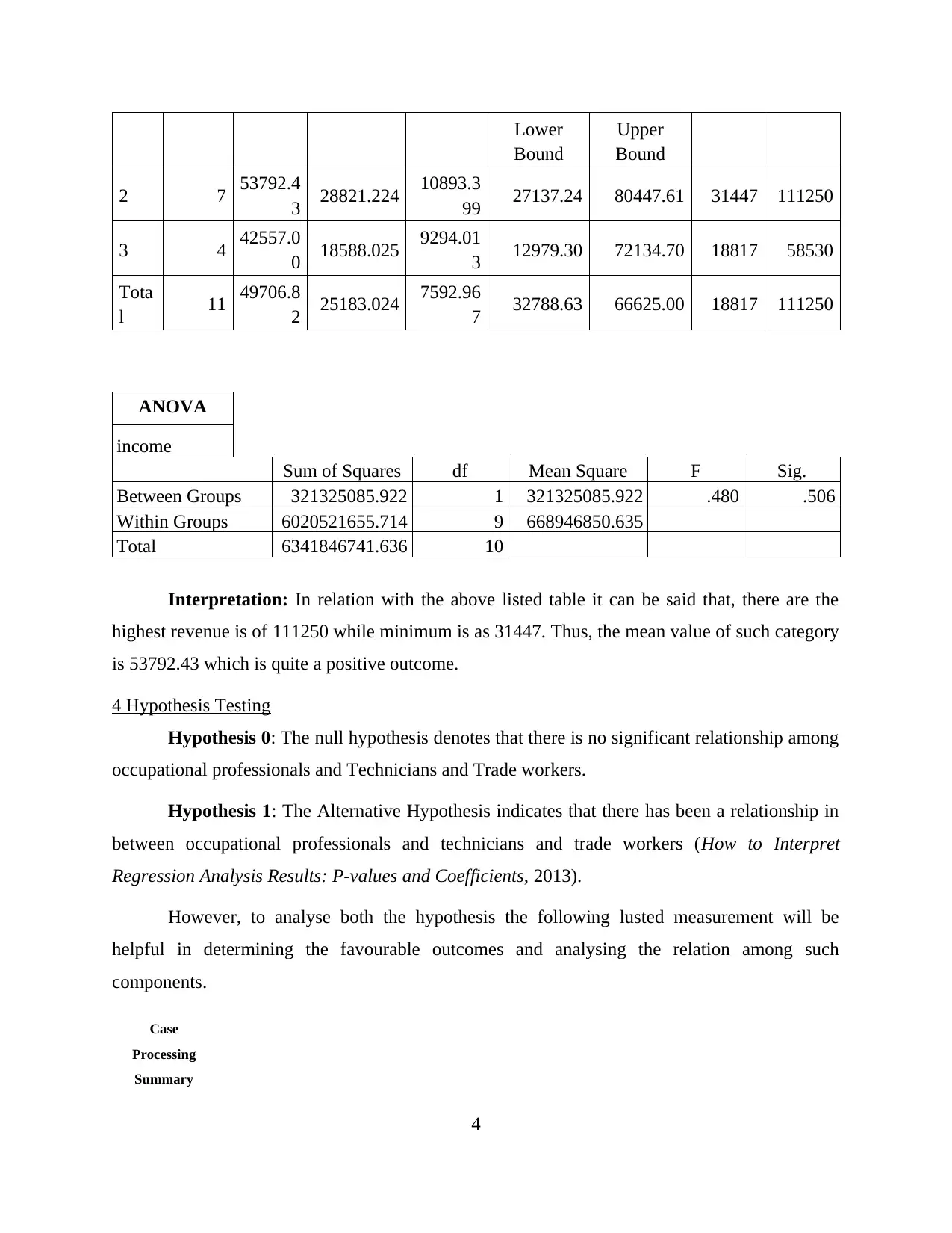
Interpretation: In relation with the above listed table it can be said that, there are the
highest revenue is of 111250 while minimum is as 31447. Thus, the mean value of such category
is 53792.43 which is quite a positive outcome.
4 Hypothesis Testing
Hypothesis 0: The null hypothesis denotes that there is no significant relationship among
occupational professionals and Technicians and Trade workers.
Hypothesis 1: The Alternative Hypothesis indicates that there has been a relationship in
between occupational professionals and technicians and trade workers (How to Interpret
Regression Analysis Results: P-values and Coefficients, 2013).
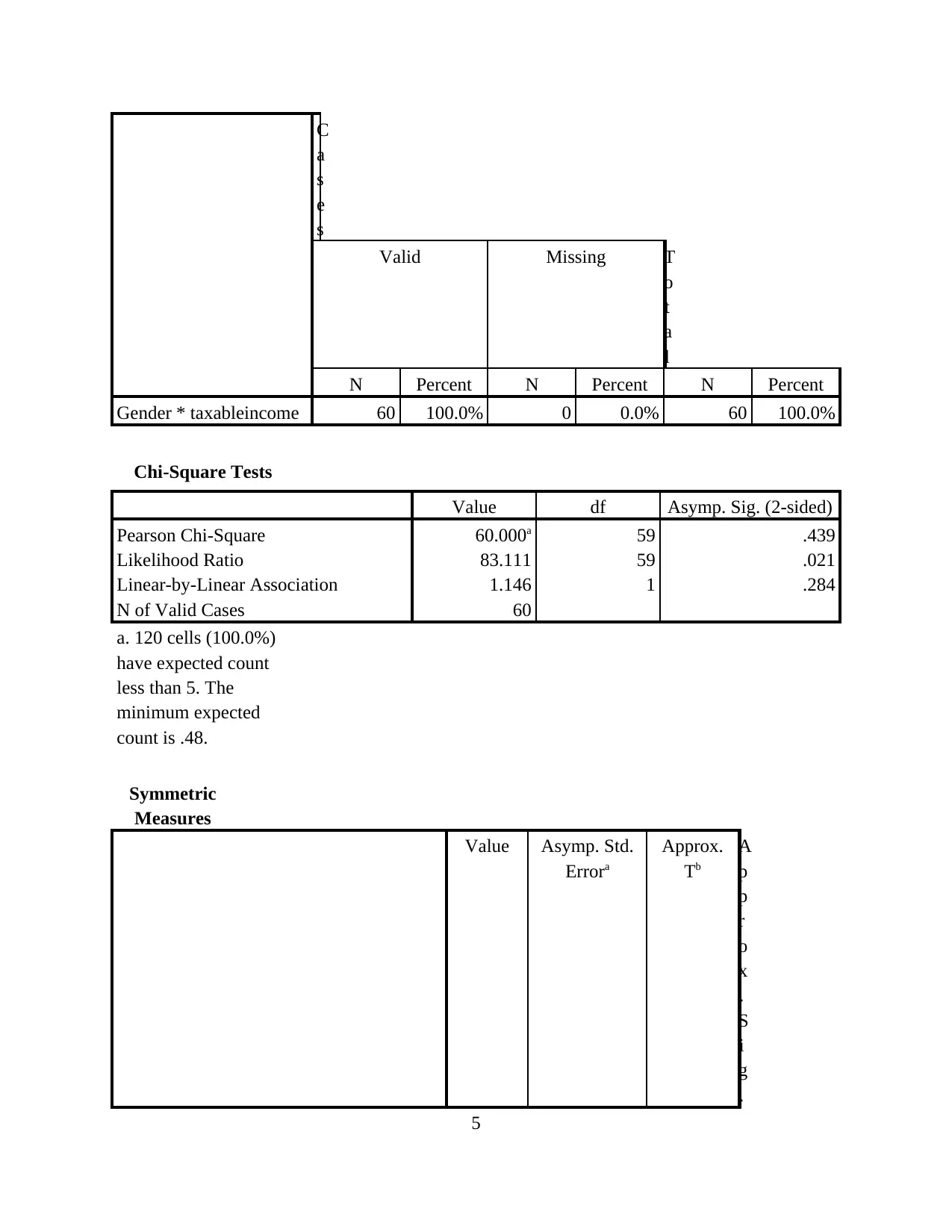
However, to analyse both the hypothesis the following lusted measurement will be
helpful in determining the favourable outcomes and analysing the relation among such
components.
Case
Processing
Summary
4

C
a
s
e
s
Valid Missing T
o
t
a
l
N Percent N Percent N Percent
Gender * taxableincome 60 100.0% 0 0.0% 60 100.0%
Chi-Square Tests
Value df Asymp. Sig. (2-sided)
Pearson Chi-Square 60.000a 59 .439
Likelihood Ratio 83.111 59 .021
Linear-by-Linear Association 1.146 1 .284
N of Valid Cases 60
a. 120 cells (100.0%)
have expected count
less than 5. The
minimum expected
count is .48.
Symmetric
Measures
Value Asymp. Std.
Errora
Approx.
Tb
A
p
p
r
o
x
.
S
i
g
.
5

Nominal by
Nominal
Phi 1.000 .439
Cramer's V 1.000 .439
Interval by Interval Pearson's R -.139 .118 -1.072 .288c
Ordinal by Ordinal Spearman
Correlation -.086 .129 -.655 .515c
N of Valid Cases 60
a. Not
assuming the
null
hypothesis.
b. Using the
asymptotic
standard error
assuming the
null
hypothesis.
c. Based on
normal
approximation
.
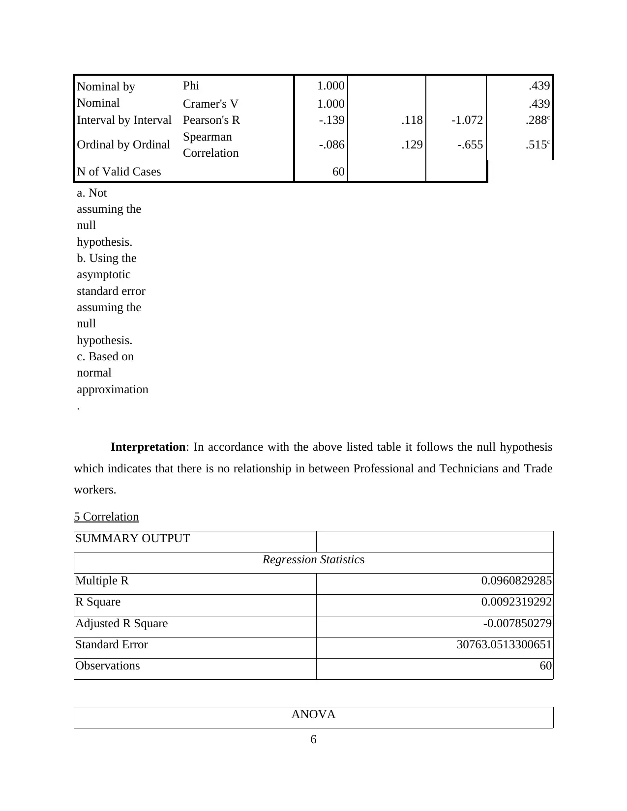
Interpretation: In accordance with the above listed table it follows the null hypothesis
which indicates that there is no relationship in between Professional and Technicians and Trade
workers.
5 Correlation
SUMMARY OUTPUT
Regression Statistics
Multiple R 0.0960829285
R Square 0.0092319292
Adjusted R Square -0.007850279
Standard Error 30763.0513300651
Observations 60
ANOVA
6

df SS MS F Significance F
Regression 1
511454818.68
2549
511454818.68
2549 0.540441206 0.4652122319
Residual 58
54889188973.
9008
946365327.13
622
Total 59
55400643792.
5833
Coefficie
nts
Standard
Error t Stat P-value
Lower
95%
Upper
95%
Lower
95.0%
Upper
95.0%
Intercept
37121.41
70040486
7357.496
4172762
5.045387
031
4.765863
62390078
E-006
22393.78
7904814
51849.04
61032832
22393.78
7904814
51849.04
61032832
age_range
942.0344
129555
1281.423
0769068
0.735147
0642
0.465212
2319
-
1623.012
5439916
3507.081
3699026
-
1623.012
5439916
3507.081
3699026
0 2 4 6 8 10 12
-100000
0
100000
200000
a g e _r a n g e R e s id u a l P lo t
a g e _ra n g e
R e s id u a ls
7

30/12/1899
0
50000
100000
150000
N o r m a l P r o b a b ilit y P lo t
C olum n P
S a m p le P e rc e n ti le
T a x a b le _I n c o m e
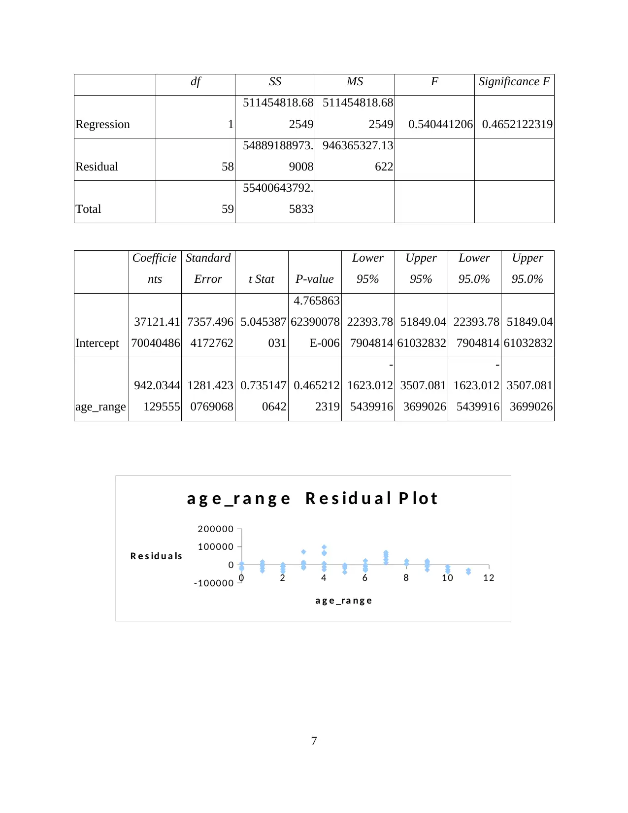
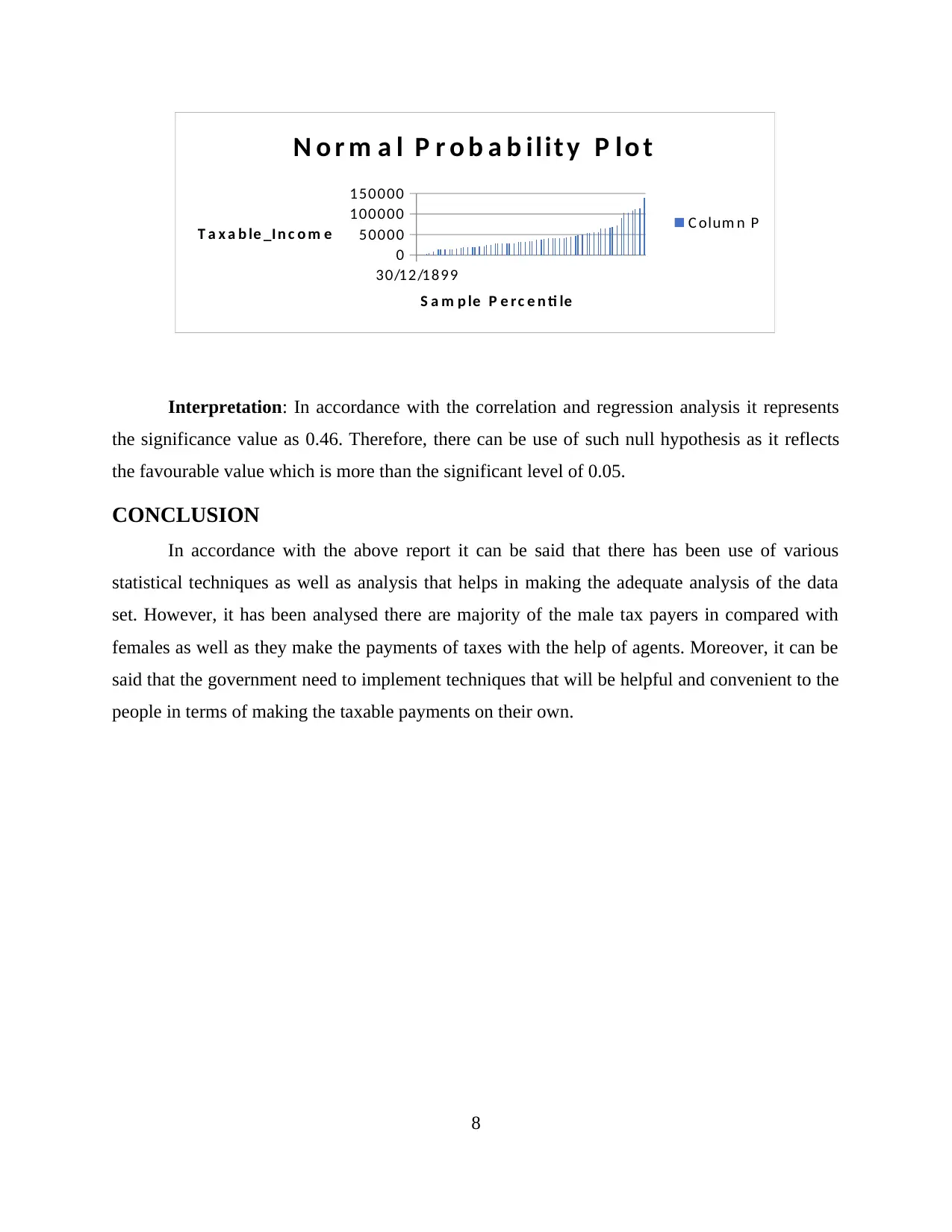
Interpretation: In accordance with the correlation and regression analysis it represents
the significance value as 0.46. Therefore, there can be use of such null hypothesis as it reflects
the favourable value which is more than the significant level of 0.05.
CONCLUSION
In accordance with the above report it can be said that there has been use of various
statistical techniques as well as analysis that helps in making the adequate analysis of the data
set. However, it has been analysed there are majority of the male tax payers in compared with
females as well as they make the payments of taxes with the help of agents. Moreover, it can be
said that the government need to implement techniques that will be helpful and convenient to the
people in terms of making the taxable payments on their own.
8

REFERENCES
Books and Journals
Olivoto, T. and et.al., 2018. Confidence Interval Width for Pearson’s Correlation Coefficient: A
Gaussian-Independent Estimator Based on Sample Size and Strength of Association.
Agronomy Journal.
Şahin, R. and Liu, P., 2017. Correlation coefficient of single-valued neutrosophic hesitant fuzzy
sets and its applications in decision making. Neural Computing and Applications. 28(6).
pp.1387-1395.
van Doorn, J. and et.al., 2018. Bayesian inference for Kendall’s rank correlation coefficient. The
American Statistician, pp.1-6.
Online
How to Interpret Regression Analysis Results: P-values and Coefficients. 2013. [Online].
Available through :<http://blog.minitab.com/blog/adventures-in-statistics-2/how-to-
interpret-regression-analysis-results-p-values-and-coefficients>.
9

APPENDIX
Appendix A
Id No unique
identifier
not applicable integer 1 to 258,774
Gender Gender (sex) Your sex question integer 0 = Male
1 = Female
Age_range Age in five
year ranges
Based on Date of Birth label, this is
their age as on 30 June 2014.
integer 0 to 11 (Table
1)
Occ_code Salary/wage
occupation
code
Income item 1, label X, first digit integer
1 to 9 (Table 2)
Lodgment_metho
d
Lodgment
method
Via tax agent, or self prepared
return.
charact
er
A(2) = Tax
Agent
S(1) = Self
Preparer
Tot_inc_amt Total income Total income or loss Dollars
WRE_Deductions Work Related
Deductions
total
Total work related deductions Dollars
Taxable_Income Taxable income
(total income
less total
deductions )
Taxable income or loss, label $ Dollars
Appendix B
Age ranges Age ranges - description
0 70 and over
1 65 to 69
2 60 to 64
3 55 to 59
10

4 50 to 54
5 45 to 49
6 40 to 44
7 35 to 39
8 30 to 34
9 25 to 29
10 20 to 24
11 under 20
Appendix C
Table 2
Occupation code (one digit level) Broad Occupation grouping
0
Occupation not listed/ Occupation not
specified
1 Managers
2 Professionals
3 Technicians and Trades Workers
4 Community and Personal Service Workers
5 Clerical and Administrative Workers
6 Sales workers
7 Machinery operators and drivers
8 Labourers
9
Consultants, apprentices and type not
specified or not listed
Appendix D
Gend
er
age_r
ange
Occ_
code
Lodgment_
method
Tot_i
nc_a
mt
WRE
Ded
Taxa
ble_I
ncom
11

e
Mean
0.483
3333
333 Mean
4.833
3333
333 Mean
4.483
33333
33 Mean 1.55 Mean
4305
1.35 Mean
1001.
9 Mean
4167
4.583
3333
333
Stand
ard
Error
0.065
0582
819
Stand
ard
Error
0.403
4922
879
Stand
ard
Error
0.405
81345
15
Standard
Error
0.064
7681
654
Stand
ard
Error
3990.
2595
8615
14
Stand
ard
Error
203.6
1018
4360
1
Stand
ard
Error
3955.
9953
7113
43
Medi
an 0
Medi
an 4.5
Medi
an 4.5 Median 2
Medi
an
3603
3.5
Medi
an 327
Medi
an
3413
4.5
Mode 0 Mode 2 Mode 0 Mode 2 Mode #N/A Mode 0 Mode #N/A
Stand
ard
Devia
tion
0.503
9392
843
Stand
ard
Devi
ation
3.125
4378
224
Stand
ard
Devi
ation
3.143
41747
88
Standard
Deviation
0.501
6920
522
Stand
ard
Devi
ation
3090
8.417
8484
175
Stand
ard
Devi
ation
1577.
1577
0628
95
Stand
ard
Devi
ation
3064
3.008
3801
535
Samp
le
Varia
nce
0.253
9548
023
Samp
le
Varia
nce
9.768
3615
819
Samp
le
Varia
nce
9.881
07344
63
Sample
Variance
0.251
6949
153
Samp
le
Varia
nce
9553
3029
3.892
373
Samp
le
Varia
nce
2487
426.4
3050
847
Samp
le
Varia
nce
9389
9396
2.586
158
Kurto
sis
-
2.065
3317
156
Kurto
sis
-
0.963
5509
535
Kurto
sis
-
1.340
21857
83 Kurtosis
-
2.026
1905
198
Kurto
sis
1.280
3541
152
Kurto
sis
11.34
3881
0261
Kurto
sis
1.360
8958
426
Skew
ness
0.068
4264
15
Skew
ness
0.259
8387
478
Skew
ness
-
0.000
62126
52 Skewness
-
0.206
1987
536
Skew
ness
1.260
9219
093
Skew
ness
2.951
6272
78
Skew
ness
1.266
7969
41
Rang
e 1
Rang
e 11
Rang
e 9 Range 1
Rang
e
1367
98
Rang
e 9074
Rang
e
1385
05
12