Inferential Statistics Analysis and Writeup

This document discusses the inferential statistics analysis plan and computation for a single head of household with two children who makes $96,664 and spends $1,478 on electricity and $18,483 on housing. The document includes confidence interval analysis and hypothesis testing. The results and write-up are also provided along with a discussion and references.

Assignment #3: Inferential Statistics Analysis and Writeup
Identifying Information
Student (Full Name):
Class:
Instructor:
Date:
Part A: Inferential Statistics Data Analysis Plan and Computation
Introduction:
The scenario: I am a single head of a household with two children who makes $96,664 and
spends$1,478 on electricity and $18,483 on housing. The variables included are Marital status
Income, Family size, Housing expense, and Electricity
Variables Selected:
Table 1: Variables Selected for Analysis
Variable Name in
the Data Set
Variable Type Description Qualitative or
Quantitative
Variable 1: Marital
status
Socioeconomic Marital status of Head of
Household
Qualitative
Variable 2: ’USD-
housing’
Expenditure Total amount annual
expenditures on Housing
Quantitative
Variable
3:’Electricity
Expense’
Expenditure Total amount of annual
expenditures on Electricity
Quantitative

Data Analysis:
1. Confidence Interval Analysis:
Table 2: Confidence Interval Information and Results
Name of Variable: ‘Housing expenditure’
State the Random Variable and Parameter in Words: The random variable is value that
vary from one person to another in this case it is housing expense. The parameter is the mean
of housing expense that is the random variable.
Confidence interval method including confidence level and rationale for using it: The
confidence interval method is usually at 95%, and it is equivalent to 5% confidence level , it
is used since it provides the chance that the true parameter value is within confidence interval
generated by the method used
State and check the assumptions for confidence interval: With 95% confidence the
population mean is between 18100 and 28500. It is also assumed that the random variable is
continuous in nature
Method Used to Analyze Data: Excel
Find the sample statistic and the confidence interval: The mean housing expense is
$21900.6 and its confidence interval is between 20499.3 and 23301.9
Statistical Interpretation: The mean housing expense for all the individual is within the
interval $20,499.3 and $23301.9. It is also evident that the population parameter is within this
interval.
2. Hypothesis Testing:
Table 3: Two Sample Hypothesis Test Analysis
Research Question: Does married and not married individual spend same amount of money in
electricity?

Two Sample Hypothesis Test that Will Be Used and Rationale for Using It: Two sample
T-test will be used. This is because marital status contained to independent categories and thus
to test the difference in expenditure of the two groups the above named test will be appropriate
State the Random Variable and Parameters in Words: The random variable will be
Electricity expense while the parameter will be T statistic
State Null and Alternative Hypotheses and Level of Significance:
H0: There is no difference in electricity expenditure between married and not married families.
H1: There is no difference in electricity expenditure between married and not married families.
Method Used to Analyze Data: Excel
Find the sample statistic, test statistic, and p-value: the t-test statistic is 2.048407 and p-
value is 0.03
Conclusion Regarding Whether or Not to Reject the Null Hypothesis:
Since the p-value is less than 5% level of significance we reject the null hypothesis that
married and not married spend same amount of money on electricity bills
Part B: Results and write up
Confidence Interval Analysis:
The results obtained revealed that average amount of household income spend on housing is
between 20499.3 and 23301.9. It means that the population average amount of spend on housing
lies within the interval.
Two Sample Hypothesis Test Analysis:
The two sample T-test statistics output generated we use to test the following hypothesis;
H0: There is no difference in electricity expenditure between married and not married families.

H1: There is no difference in electricity expenditure between married and not married families.
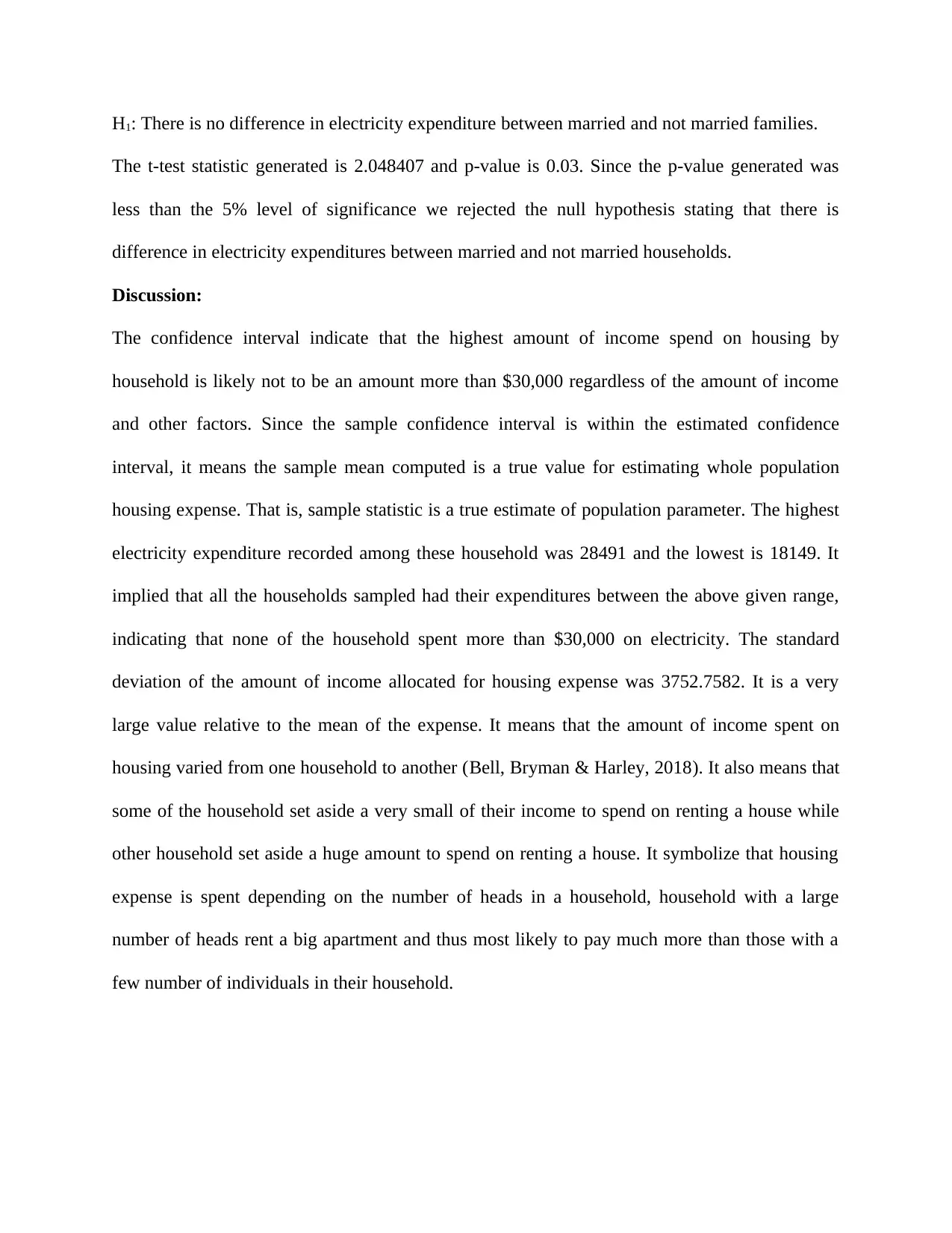
The t-test statistic generated is 2.048407 and p-value is 0.03. Since the p-value generated was
less than the 5% level of significance we rejected the null hypothesis stating that there is
difference in electricity expenditures between married and not married households.
Discussion:
The confidence interval indicate that the highest amount of income spend on housing by
household is likely not to be an amount more than $30,000 regardless of the amount of income
and other factors. Since the sample confidence interval is within the estimated confidence
interval, it means the sample mean computed is a true value for estimating whole population
housing expense. That is, sample statistic is a true estimate of population parameter. The highest
electricity expenditure recorded among these household was 28491 and the lowest is 18149. It
implied that all the households sampled had their expenditures between the above given range,
indicating that none of the household spent more than $30,000 on electricity. The standard
deviation of the amount of income allocated for housing expense was 3752.7582. It is a very
large value relative to the mean of the expense. It means that the amount of income spent on
housing varied from one household to another (Bell, Bryman & Harley, 2018). It also means that
some of the household set aside a very small of their income to spend on renting a house while
other household set aside a huge amount to spend on renting a house. It symbolize that housing
expense is spent depending on the number of heads in a household, household with a large
number of heads rent a big apartment and thus most likely to pay much more than those with a
few number of individuals in their household.

The two groups of people had different standard deviations. The individuals who were not
married had electricity expense which has a standard deviation of 14.2137. This is a very small
value, indicating that the variation of amount of income allocated for electricity was very little
and thus majority of the households who are not married spent almost the same amount on
expense. On the other hand, household who are married had a standard deviation of 110.4256. It
is a very huge value compared to that of not married households. It implies that majority of the
amount of income spent by married household had a very huge dispersion. The value is far much
more than that of household who are not married. It might be because of the fact that married
household had a varied number of individuals per household. It also means that some of the
married household pay very little amount for electricity bills while also a good number of them
pay a relatively huge amount of electricity expense.
We concluded that indeed there is difference in the amount of income allocated for electricity
between married household and not married household. It means that one category of the
households either spend lower or higher than another group. The average electricity expense for
married household is $1399.667 while that of not married household is $1462.8. This means that
not married household spent more income on electricity bills compared to their counterpart
married who spend the above. This might be because they incur less expense not married use a
lot of electrical appliances which will lead to more consumption of electricity by the devices.

References
Bell, E., Bryman, A., & Harley, B. (2018). Business research methods. New York:Oxford
university press.
Murray R Spiegel & John J Schiller. (2009). Probability and statistics. New York: Mcgraw-hill.