Numerical Solutions of Riccati Equation | PDF
VerifiedAdded on 2021/10/01
|57
|7256
|150
AI Summary
Contribute Materials
Your contribution can guide someone’s learning journey. Share your
documents today.
Bachelor of Science (Hons.) Mathematics
Center of Mathematics Studies Faculty of Computer and Mathematical
Sciences
TECHNICAL REPORT
NUMERICAL SOLUTIONS OF RICCATI EQUATIONS USING
ADAM-BASHFORTH AND ADAM-MOULTON METHODS
MOHAMAD NAZRI BIN MOHAMAD KHATA 2014885526
NUR HABIBAH BINTI RADZALI 2014246052
MOHAMAD ALIFF AFIFUDDIN BIN HILMY 2014675202
K162/15
Secure Best Marks with AI Grader
Need help grading? Try our AI Grader for instant feedback on your assignments.
UNIVERSITI TEKNOLOGI MARA
TECHNICAL REPORT
NUMERICAL SOLUTIONS OF RICCATI
EQUATIONS USING ADAM-BASHFORTH AND
ADAM-MOULTON METHODS
MOHAMAD NAZRI BIN MOHAMAD KHATA
2014885526 CS2495C
NUR HABIBAH BINTI RADZALI
2014246052 CS2495C
MOHAMAD ALIFF AFIFUDDIN BIN HILMY
2014675202 CS2495C
Report submitted in partial fulfillment of the requirement
for the degree of
Bachelor of Science (Hons.) Mathematics
Center of Mathematics Studies
Faculty of Computer and Mathematical Sciences
JULY 2017

ACKNOWLEDGEMENTS
IN THE NAME OF ALLAH, THE MOST GRACIOUS, THE MOST MERCIFUL
Firstly, we are grateful to Allah S.W.T for giving us the strength to complete this project
successfully. We would like to express our gratitude to all people involved in our final year
project. Throughout the process, we are in contact with many lecturers and friends. They have
contributed in their own way towards ours understanding and thoughts about the whole research
project.
We also would like to express our deepest gratitude and appreciation to the our beloved
supervisor, Miss Farahanie binti Fauzi, for her valuable time, advices and the guidance that we
need to complete our project from the beginning up to the end of the writing. To all lecturers
and friends who have willingly sacrificed their time to help us, we want to record or sincere
thanks.
In addition, we are also indebted to all our undergraduate friends who have helped us
by giving brilliant ideas. Our sincere appreciation also extends to those who have provided
assistance at various occasions. Their views and tips are useful indeed.
Last but not least, we would like to thanks to our beloved parents for their continuous
encouragement and supports for our team. Without their support it would be hard for us to
finish this study.
ii
TABLE OF CONTENTS
ACKNOWLEDGEMENTS ii
TABLE OF CONTENTS iii
LIST OF FIGURES v
LIST OF TABLES vi
ABSTRACT vii
1 INTRODUCTION 1
1.1 Problem Statement 3
1.2 Research Objective 3
1.3 Significant Of Project 4
1.4 Scope Of Project 4
2 LITERATURE REVIEW 5
3 METHODOLOGY 7
3.1 Introduction of Adam-Bashforth and Adam-Moulton Methods 7
3.2 Introduction to Riccati Equation 9
3.3 Accuracy of Analysis 11
3.4 Analysis of apply both Adam-Bashforth and Moulton methods 11
4 IMPLEMENTATION 12
4.1 Derivation of Adam-Bashforth and Adam-Moulton Methods 12
4.2 Solving Riccati Equation 20
4.3 Analysis of Results Obtained 23
5 RESULTS AND DISCUSSION 25
iii
Secure Best Marks with AI Grader
Need help grading? Try our AI Grader for instant feedback on your assignments.
5.1 Result 25
5.2 Discussion 26
6 CONCLUSIONS AND RECOMMENDATIONS 27
REFERENCES 28
iv
5.2 Discussion 26
6 CONCLUSIONS AND RECOMMENDATIONS 27
REFERENCES 28
iv

LIST OF FIGURES
Figure 4.1 Coding of Adam Bashforth 21
Figure 4.2 Coding of Adam Moulton 22
v
Figure 4.1 Coding of Adam Bashforth 21
Figure 4.2 Coding of Adam Moulton 22
v
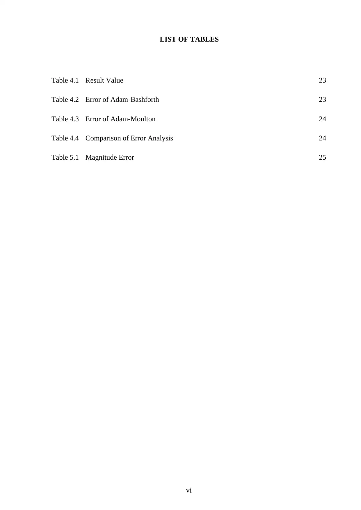
LIST OF TABLES
Table 4.1 Result Value 23
Table 4.2 Error of Adam-Bashforth 23
Table 4.3 Error of Adam-Moulton 24
Table 4.4 Comparison of Error Analysis 24
Table 5.1 Magnitude Error 25
vi
Table 4.1 Result Value 23
Table 4.2 Error of Adam-Bashforth 23
Table 4.3 Error of Adam-Moulton 24
Table 4.4 Comparison of Error Analysis 24
Table 5.1 Magnitude Error 25
vi
Paraphrase This Document
Need a fresh take? Get an instant paraphrase of this document with our AI Paraphraser
ABSTRACT
A differential equation can be solved analytically or numerically. In many complicated
cases, it is enough to just approximate the solution if the differential equation cannot be solved
analytically. Euler’s method, the improved Euler’s method and Runge-Kutta methods are ex-
amples of commonly used numerical techniques in approximately solved differential equations.
These methods are also called as single-step methods or starting methods because they use the
value from one starting step to approximate the solution of the next step. While, multistep or
continuing methods such as Adam-Bashforth and Adam-Moulton methods use the values from
several computed steps to approximate the value of the next step. So, in terms of minimizing
the calculating time in solving differential , multistep method is recommended by previous re-
searchers.In this project, a Riccati differential equation is solved using the two multistep meth-
ods in order to analyze the accuracy of both methods. Both methods give small errors when
they are compared to the exact solution but it is identified that Adam-Bashforth method is more
accurate than Adam-Moulton method.
vii
1 INTRODUCTION
It has been shown that a solution of a differential equation exist in certain specified domain.
But in many instances, it is enough to just approximate the solution if the differential equation
cannot be solved analytically. Euler’s method, the improved Euler’s method and Runge-Kutta
methods are examples of commonly used numerical techniques in approximately solved dif-
ferential equations. These methods are also called as single-step methods or starting methods
because they use the value from one starting step to approximate the solution of the next step.
In the other hand, multistep or continuing methods such as Adam-Bashforth and Adam-
Moulton methods use the values from several computed steps to approximate the value of the
next step. Since linear multistep methods need several starting values to compute the next value,
it is necessary to use a one-step method to compute enough its’ starting values of the solution
in order to be used in the multistep method.
First-order numerical procedure for solving ordinary differential equations (ODEs) like
Euler method with a given initial value. Simplest Runge–Kutta method is the custom of basic
explicit method for numerical integration in an ordinary differential equations. Euler method
refers to only one previous point and its derivative to determine the current value. A simple
modification of the Euler method which eliminates the stability problems is the backward Euler
method. This modification leads to a family of Runge-Kutta.
Runge–Kutta methods are a family of implicit and explicit iterative methods, which in-
cludes the well-known routine called the Euler Method. The most popular and widely used is
RK4 because its less computational requirement and high accuracy. This RK4 is an example of
one-step method in numerical, Petzoldf (1986). Development of modified this RK4 leads from
one-step to multi-step method,like Adam’s methods.
Adam-Bashforth method and Adam-Moulton methods are the families of linear multistep
method that commonly used. Adam-Bashforth methods is an example of explicit methods of
1
multi-step, Garrappa (2009). Adam Bashforth method are designed by John Couch Adams
to solve a differential equation modeling capillary action due to Francis Bashforth, Misirli &
Gurefe (2011)
While Adam-Moulton methods is an example of implicit methods. The backward Euler
method can also be seen as a linear multistep method with one step. It is the first method of
the family of Adams–Moulton methods, and also of the family of backward differentiation for-
mulas. Adam-Moulton methods are solely due to John Couch Adam, just like Adam-Bashforth
method. The name of Forest Ray Moulton become associated with these methods because he re-
alized that they could be used in tandem with Adam-Bashforth Method as a predictor-corrector
pair. Jator (2001)
Non-linear differential equation are commonly used in spring mass system, resistor capac-
itor induction and many more. A part of this non-linear is Riccati differential equation which is
well-known among them. This equation is named after Jacopo Francesco Riccati. Solution of
Riccati equation is usually solved by two numerical technique which are cubic B-spline scaling
function and Chebyshev cardinal function and also used to refer to matrix equation are shown in
File & Aga (2016). Riccati equation play a fundamental role in financial mathematics, network
synthesis and optimal control.Ghomanjani & Khorram (2017)
2
Secure Best Marks with AI Grader
Need help grading? Try our AI Grader for instant feedback on your assignments.
1.1 Problem Statement
Basically, single-step methods especially Runge-Kutta method is often used because of its ac-
curacy. However, the process of calculation is time consuming since the differential equation
need to be evaluated several times at every step. For example, the Runge-Kutta of order 4 (RK4)
method requires four functions evaluation for every step. Otherwise, a multistep method need
only one new function to evaluate for every step. So, it is best to apply multistep method to
solve differential equations in order to reduce the time required in the calculation process.
1.2 Research Objective
The purpose of this project are
1. To derive 4-steps Adam-Bashforth and Adam Moulton methods using Maple Software
2. To apply 4-steps of Adam-Bashforth and Adam-Moulton in solving Riccati Equation by
using Matlab
3. To analyse the accuracy of 4-steps Adam-Bashforth and Adam-Moulton on Riccati
Equation
3
1.3 Significant Of Project
This topic is chosen because some people only know how to approximate value using basis
methods. By using this linear multi-step method, other mathematicians will understand that
there a better and easier way to approximate a value. Furthermore, it will inspire new mathe-
maticians to invent new formula that can be derived from an old formula.
1.4 Scope Of Project
This project focused on solving Riccati differential equations by using numerical methods
which are Adam-Bashforth and Adam-Moulton method. Deriving the 4-step of both methods
require Maple application while the final result of Riccati equation require Matlab application.
The combination of both applications provide easier way to solve the Riccati differential equa-
tions.
4
2 LITERATURE REVIEW
Adam-Bashforth and Adam-Moulton are explicit/implicit numerical integration. Both methods
can solve as an approximation in nonlinear differential equation. Traditional Adam-Bashforth-
Moulton predictor-corrector method is proposed long ago and since then the methods have been
continuously improved.
Adam Bashforth was derived explicitly using Newton Backward Difference Formula with
an equal of spacing points. In order to differenciate Adam Bashforth and Adam Moulton
Method, the mathematician proposed the use of m-step for Adam Bashforth and m-1 for Adam
Moulton. As a conclusion, both method are already derived by Chiou & Wu (1999).
Then according Aboiyar et al. (2015) solving first order initial value problems (IVPs) of
ordinary differential equation with step number m=3. This journal using Hermite polynomials
as basis function. Using the collocation and interpolation technique Adam-Bashforth, Adam-
Moulton and Optimal Order Method was invented. Then to derive 3-step of Adam-Bashforth
is set n=3 and Adam Moulton is sets n=4 in equation probabilist’s Hermite polynomial. As a
conclusion, the best result was obtained and been compared to see which method give the best
approximation with less of error.
Furthermore, a direct solution can be developed by using Adam-Moulton methods comes
from Jator (2001). This solution must be used to calculate the initial value problem. As from
Areo & Adeniyi (2013) ,the solution is in the form of first derivatives of y in terms of x and
y. There is range for x which is [a,b] and it’s a finite real number. Therefore the solution is
the form of first derivative before a unique solution. For general linear multistep method of
step k, the derivatives y only need to be evaluate a few times which is less than the number of
evaluations for the one-step method in the range of integration [a,b]. So by Butcher (2000) it is
proof that the linear multistep method is better than one-step method.
5
Paraphrase This Document
Need a fresh take? Get an instant paraphrase of this document with our AI Paraphraser
Regarding Anake & Ashibel Cugp (2011) one step methods include the Euler’s methods,
the Runge-Kutta methods and the theta methods. These methods are only suitable for the so-
lutions of first order IVPs of ODEs because of their very low order of accuracy which say by
C Butcher John (1987). However, by Petzoldf (1986) in order to develop higher order one step
methods such as Runge-Kutta methods, the efficiency of Euler methods in terms of the number
of function evaluations per step is sacrificed since more function evaluations is required.
On the other hand of linear multistep methods, include methods such as Adam-Bashforth
method, Adam-Moulton method, and Numerov method. These methods give high order of
accuracy and are suitable without necessarily reducing it to an equivalent system of first order
IVPs of ODEs. Linear multistep methods are not as efficient, in terms of function evaluations,
as the one step method and also require some values to start the integration process.
Various method are used to solve the Riccati differential equation and one of it is Bezier
curves. In that method, the Bezier polynomial of degree n is develop and new efficient method,
the multistage variational iteration is applied. File & Aga (2016) said that many authors are
working with the Bezier curves. Some of them use Bezier control point in approximating date
and function while some are using it to solve differential equation numerically.
In addition, solving delay differential equation and singular perturbed two points boundary
value problems are also using Bezier curves. Amman & Neudecker (1997) pointed out that
solving the riccati equation recursively in time is simple which generally doesn’t pose any
difficulties.
Finally, one of class in nonlinear equation are Riccati differential equation and have played
many roles in applied science. One-dimensional static Schrödinger equation is closely related
to the Riccati differential equation. The Riccati differential equation is named after the Ital-
ian nobleman Count Jacopo Francesco Riccati(1676–1754). The applications of this equation
maybe found not only in random processes, optimal control, and diffusion problems but also in
stochastic realization theory, optimal control, network synthesis and financial mathematics.
6
3 METHODOLOGY
This section is divided into 4 subsections. In the first subsection, the introduction to Adam-
Bashforth and Adam-Moulton Methods are stated and in the second subsection, the introduction
of Riccati Equation is then stated. In the third subsection, a little explanation on how to derive
a higher step Adam-Bashforth and Adam-Moulton is discussed. Last but not least, the process
of analyzing the accuracy of Adam-Bashforth and Adam-Moulton methods is discussed in the
final subsection.
3.1 Introduction of Adam-Bashforth and Adam-Moulton Methods
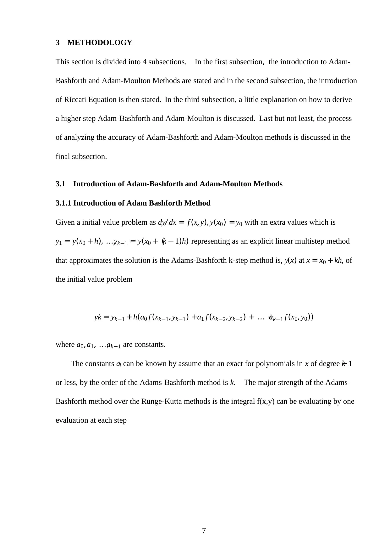
3.1.1 Introduction of Adam Bashforth Method
Given a initial value problem as dy/ dx = f (x,y),y(x0) =y0 with an extra values which is
y1 = y(x0 +h), ...,yk−1 = y(x0 + (k − 1)h) representing as an explicit linear multistep method
that approximates the solution is the Adams-Bashforth k-step method is, y(x) at x = x0 +kh, of
the initial value problem
yk = yk−1 +h(a0 f (xk−1,yk−1) +a1 f (xk−2,yk−2) + ... +ak−1 f (x0,y0))
where a0,a1, ...,ak−1 are constants.
The constants ai can be known by assume that an exact for polynomials in x of degree k−1
or less, by the order of the Adams-Bashforth method is k. The major strength of the Adams-
Bashforth method over the Runge-Kutta methods is the integral f(x,y) can be evaluating by one
evaluation at each step
7
This section is divided into 4 subsections. In the first subsection, the introduction to Adam-
Bashforth and Adam-Moulton Methods are stated and in the second subsection, the introduction
of Riccati Equation is then stated. In the third subsection, a little explanation on how to derive
a higher step Adam-Bashforth and Adam-Moulton is discussed. Last but not least, the process
of analyzing the accuracy of Adam-Bashforth and Adam-Moulton methods is discussed in the
final subsection.
3.1 Introduction of Adam-Bashforth and Adam-Moulton Methods
3.1.1 Introduction of Adam Bashforth Method
Given a initial value problem as dy/ dx = f (x,y),y(x0) =y0 with an extra values which is
y1 = y(x0 +h), ...,yk−1 = y(x0 + (k − 1)h) representing as an explicit linear multistep method
that approximates the solution is the Adams-Bashforth k-step method is, y(x) at x = x0 +kh, of
the initial value problem
yk = yk−1 +h(a0 f (xk−1,yk−1) +a1 f (xk−2,yk−2) + ... +ak−1 f (x0,y0))
where a0,a1, ...,ak−1 are constants.
The constants ai can be known by assume that an exact for polynomials in x of degree k−1
or less, by the order of the Adams-Bashforth method is k. The major strength of the Adams-
Bashforth method over the Runge-Kutta methods is the integral f(x,y) can be evaluating by one
evaluation at each step
7
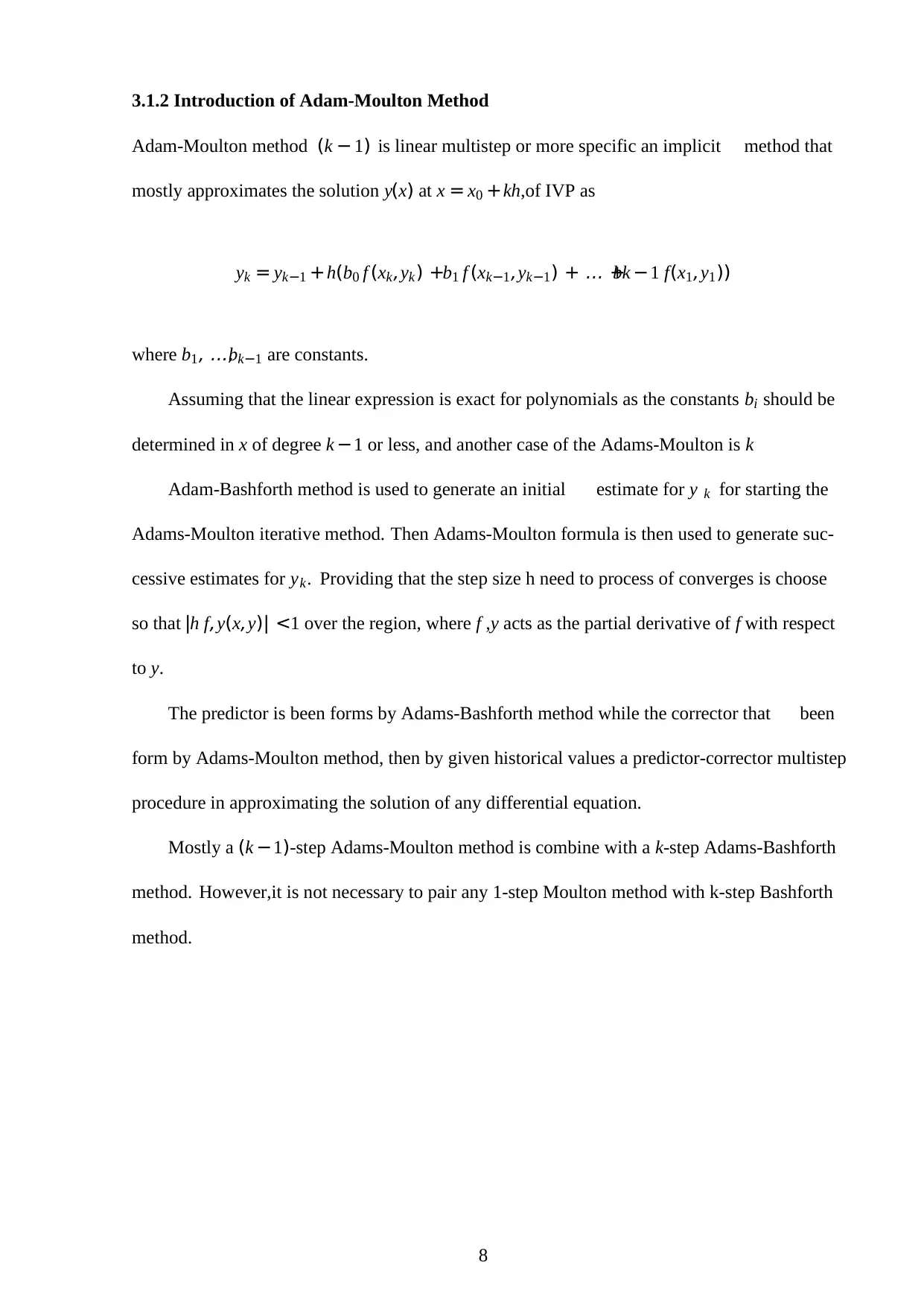
3.1.2 Introduction of Adam-Moulton Method
Adam-Moulton method (k − 1) is linear multistep or more specific an implicit method that
mostly approximates the solution y(x) at x = x0 +kh,of IVP as
yk = yk−1 +h(b0 f (xk,yk) +b1 f (xk−1,yk−1) + ... +bk −1 f(x1,y1))
where b1, ...,bk−1 are constants.
Assuming that the linear expression is exact for polynomials as the constants bi should be
determined in x of degree k −1 or less, and another case of the Adams-Moulton is k
Adam-Bashforth method is used to generate an initial estimate for y k for starting the
Adams-Moulton iterative method. Then Adams-Moulton formula is then used to generate suc-
cessive estimates for yk. Providing that the step size h need to process of converges is choose
so that |h f,y(x,y)| <1 over the region, where f ,y acts as the partial derivative of f with respect
to y.
The predictor is been forms by Adams-Bashforth method while the corrector that been
form by Adams-Moulton method, then by given historical values a predictor-corrector multistep
procedure in approximating the solution of any differential equation.
Mostly a (k −1)-step Adams-Moulton method is combine with a k-step Adams-Bashforth
method. However,it is not necessary to pair any 1-step Moulton method with k-step Bashforth
method.
8
Secure Best Marks with AI Grader
Need help grading? Try our AI Grader for instant feedback on your assignments.
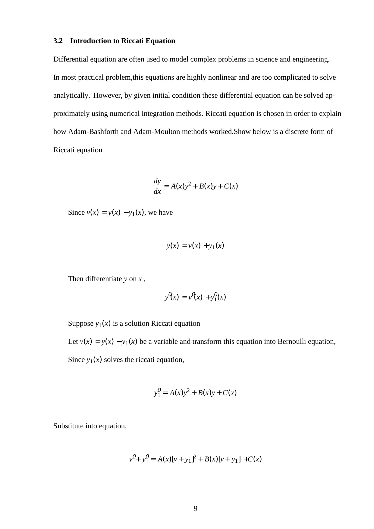
3.2 Introduction to Riccati Equation
Differential equation are often used to model complex problems in science and engineering.
In most practical problem,this equations are highly nonlinear and are too complicated to solve
analytically. However, by given initial condition these differential equation can be solved ap-
proximately using numerical integration methods. Riccati equation is chosen in order to explain
how Adam-Bashforth and Adam-Moulton methods worked.Show below is a discrete form of
Riccati equation
dy
dx = A(x)y2 +B(x)y +C(x)
Since v(x) =y(x) −y1(x), we have
y(x) =v(x) +y1(x)
Then differentiate y on x ,
y0
(x) =v0
(x) +y0
1(x)
Suppose y1(x) is a solution Riccati equation
Let v(x) =y(x) −y1(x) be a variable and transform this equation into Bernoulli equation,
Since y1(x) solves the riccati equation,
y0
1 = A(x)y2 +B(x)y +C(x)
Substitute into equation,
v0+y0
1 = A(x)[v +y1]2 +B(x)[v +y1] +C(x)
9
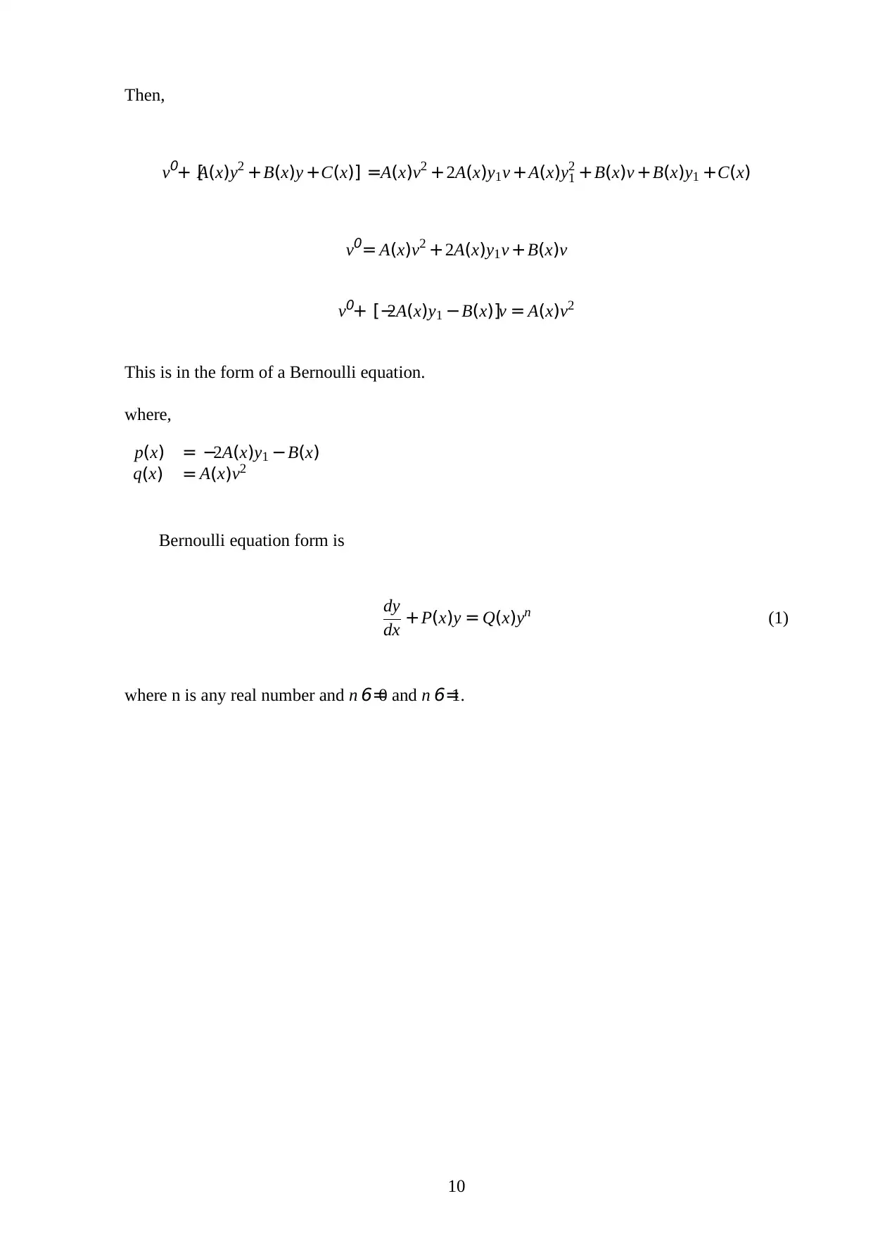
Then,
v0+ [A(x)y2 +B(x)y +C(x)] =A(x)v2 +2A(x)y1v +A(x)y2
1 +B(x)v +B(x)y1 +C(x)
v0= A(x)v2 +2A(x)y1v +B(x)v
v0+ [−2A(x)y1 −B(x)]v = A(x)v2
This is in the form of a Bernoulli equation.
where,
p(x) = −2A(x)y1 −B(x)
q(x) = A(x)v2
Bernoulli equation form is
dy
dx +P(x)y = Q(x)yn (1)
where n is any real number and n 6=0 and n 6=1.
10
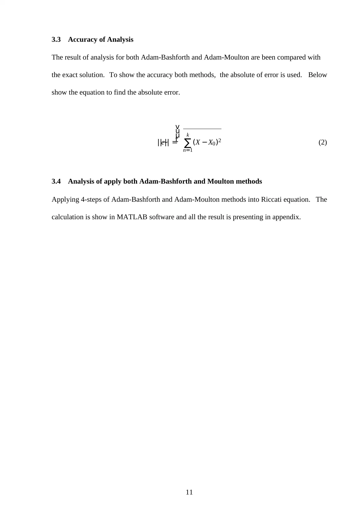
3.3 Accuracy of Analysis
The result of analysis for both Adam-Bashforth and Adam-Moulton are been compared with
the exact solution. To show the accuracy both methods, the absolute of error is used. Below
show the equation to find the absolute error.
||~e|| =
v
u
u
t k
∑
n=1
(X −X0)2 (2)
3.4 Analysis of apply both Adam-Bashforth and Moulton methods
Applying 4-steps of Adam-Bashforth and Adam-Moulton methods into Riccati equation. The
calculation is show in MATLAB software and all the result is presenting in appendix.
11
Paraphrase This Document
Need a fresh take? Get an instant paraphrase of this document with our AI Paraphraser
4 IMPLEMENTATION
In this section, will show all the calculation and derivation of the equation. As from 3.1, how
Adam-Bashforth and Adam-Moulton are formed into methods. Continuing in 4.1 is derivation
of Adam-Bashforth Method with n = 4. In 4.2 is show derivation of Adam-Moulton Method
with n = 5. Both this method are derived by using Maple 15.
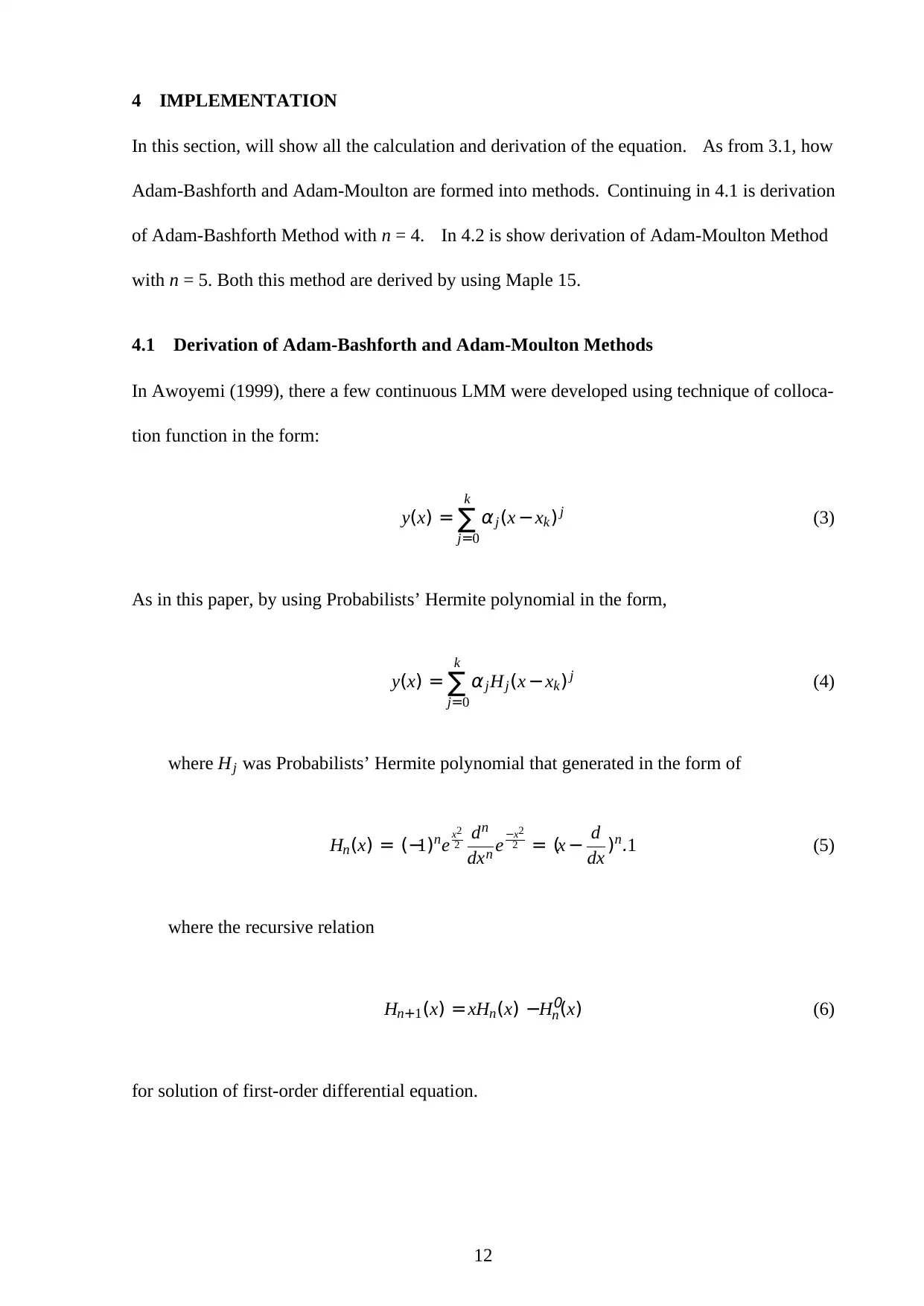
4.1 Derivation of Adam-Bashforth and Adam-Moulton Methods
In Awoyemi (1999), there a few continuous LMM were developed using technique of colloca-
tion function in the form:
y(x) =
k
∑
j=0
αj(x −xk) j (3)
As in this paper, by using Probabilists’ Hermite polynomial in the form,
y(x) =
k
∑
j=0
αjHj(x −xk) j (4)
where Hj was Probabilists’ Hermite polynomial that generated in the form of
Hn(x) = (−1)ne x2
2 dn
dxn e−x2
2 = (x − d
dx )n.1 (5)
where the recursive relation
Hn+1(x) =xHn(x) −H0
n(x) (6)
for solution of first-order differential equation.
12
In this section, will show all the calculation and derivation of the equation. As from 3.1, how
Adam-Bashforth and Adam-Moulton are formed into methods. Continuing in 4.1 is derivation
of Adam-Bashforth Method with n = 4. In 4.2 is show derivation of Adam-Moulton Method
with n = 5. Both this method are derived by using Maple 15.
4.1 Derivation of Adam-Bashforth and Adam-Moulton Methods
In Awoyemi (1999), there a few continuous LMM were developed using technique of colloca-
tion function in the form:
y(x) =
k
∑
j=0
αj(x −xk) j (3)
As in this paper, by using Probabilists’ Hermite polynomial in the form,
y(x) =
k
∑
j=0
αjHj(x −xk) j (4)
where Hj was Probabilists’ Hermite polynomial that generated in the form of
Hn(x) = (−1)ne x2
2 dn
dxn e−x2
2 = (x − d
dx )n.1 (5)
where the recursive relation
Hn+1(x) =xHn(x) −H0
n(x) (6)
for solution of first-order differential equation.
12
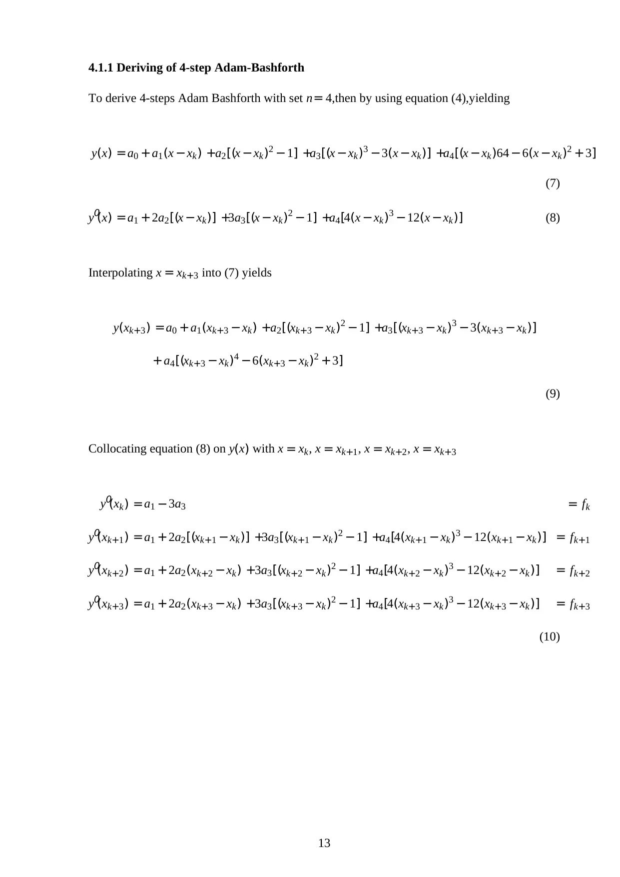
4.1.1 Deriving of 4-step Adam-Bashforth
To derive 4-steps Adam Bashforth with set n= 4,then by using equation (4),yielding
y(x) =a0 +a1(x −xk) +a2[(x −xk)2 −1] +a3[(x −xk)3 −3(x −xk)] +a4[(x −xk)64 −6(x −xk)2 +3]
(7)
y0
(x) =a1 +2a2[(x −xk)] +3a3[(x −xk)2 −1] +a4[4(x −xk)3 −12(x −xk)] (8)
Interpolating x = xk+3 into (7) yields
y(xk+3) =a0 +a1(xk+3 −xk) +a2[(xk+3 −xk)2 −1] +a3[(xk+3 −xk)3 −3(xk+3 −xk)]
+a4[(xk+3 −xk)4 −6(xk+3 −xk)2 +3]
(9)
Collocating equation (8) on y(x) with x = xk, x = xk+1, x = xk+2, x = xk+3
y0
(xk) =a1 −3a3 = fk
y0
(xk+1) =a1 +2a2[(xk+1 −xk)] +3a3[(xk+1 −xk)2 −1] +a4[4(xk+1 −xk)3 −12(xk+1 −xk)] = fk+1
y0
(xk+2) =a1 +2a2(xk+2 −xk) +3a3[(xk+2 −xk)2 −1] +a4[4(xk+2 −xk)3 −12(xk+2 −xk)] = fk+2
y0
(xk+3) =a1 +2a2(xk+3 −xk) +3a3[(xk+3 −xk)2 −1] +a4[4(xk+3 −xk)3 −12(xk+3 −xk)] = fk+3
(10)
13
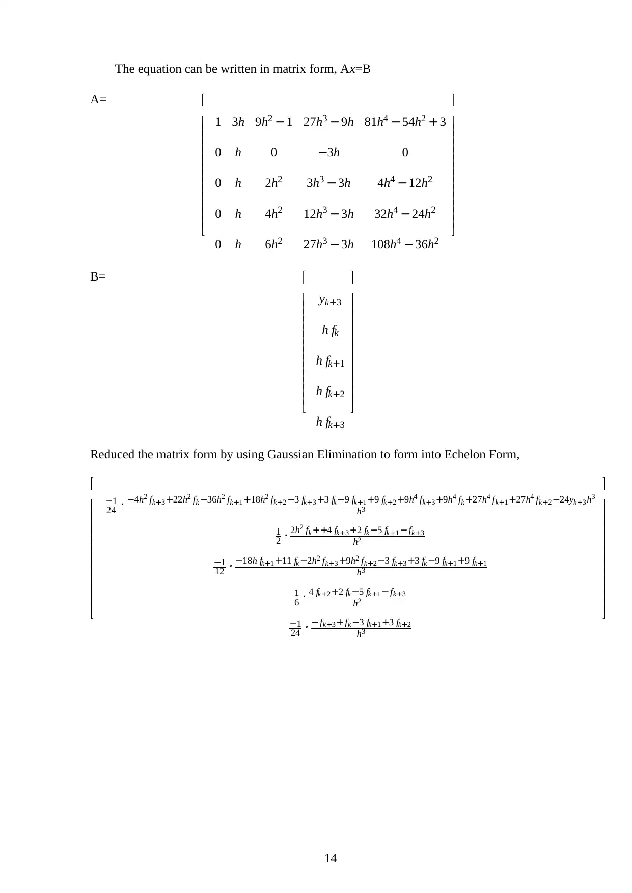
The equation can be written in matrix form, Ax=B
A=
1 3h 9h2 −1 27h3 −9h 81h4 −54h2 +3
0 h 0 −3h 0
0 h 2h2 3h3 −3h 4h4 −12h2
0 h 4h2 12h3 −3h 32h4 −24h2
0 h 6h2 27h3 −3h 108h4 −36h2
B=
yk+3
h fk
h fk+1
h fk+2
h fk+3
Reduced the matrix form by using Gaussian Elimination to form into Echelon Form,
−1
24 · −4h2 fk+3+22h2 fk−36h2 fk+1+18h2 fk+2−3 fk+3+3 fk−9 fk+1+9 fk+2+9h4 fk+3+9h4 fk+27h4 fk+1+27h4 fk+2−24yk+3h3
h3
1
2 · 2h2 fk++4 fk+3+2 fk−5 fk+1−fk+3
h2
−1
12 · −18h fk+1+11 fk −2h2 fk+3+9h2 fk+2−3 fk+3+3 fk−9 fk+1+9 fk+1
h3
1
6 · 4 fk+2+2 fk−5 fk+1−fk+3
h2
−1
24 · −fk+3+fk−3 fk+1+3 fk+2
h3
14
Secure Best Marks with AI Grader
Need help grading? Try our AI Grader for instant feedback on your assignments.
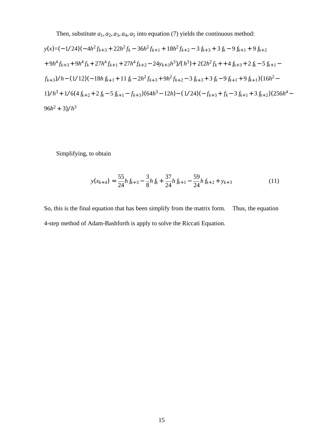
Then, substitute a1,a2,a3,a4,a5 into equation (7) yields the continuous method:
y(x)=(−1/ 24)(−4h2 fk+3 +22h2 fk −36h2 fk+1 +18h2 fk+2 −3 fk+3 +3 fk −9 fk+1 +9 fk+2
+9h4 fk+3 +9h4 fk +27h4 fk+1 +27h4 fk+2 −24yk+3h3)/( h3)+ 2(2h2 fk ++4 fk+3 +2 fk −5 fk+1 −
fk+3)/ h−(1/ 12)(−18h fk+1 +11 fk −2h2 fk+3 +9h2 fk+2 −3 fk+3 +3 fk −9 fk+1 +9 fk+1)(16h2 −
1)/ h3 +1/ 6(4 fk+2 +2 fk −5 fk+1 − fk+3)(64h3 −12h)−(1/ 24)(−fk+3 + fk −3 fk+1 +3 fk+2)(256h4 −
96h2 +3)/ h3
Simplifying, to obtain
y(xk+4) = 55
24h fk+3 − 3
8h fk + 37
24h fk+1 − 59
24h fk+2 +yk+3 (11)
So, this is the final equation that has been simplify from the matrix form. Thus, the equation
4-step method of Adam-Bashforth is apply to solve the Riccati Equation.
15
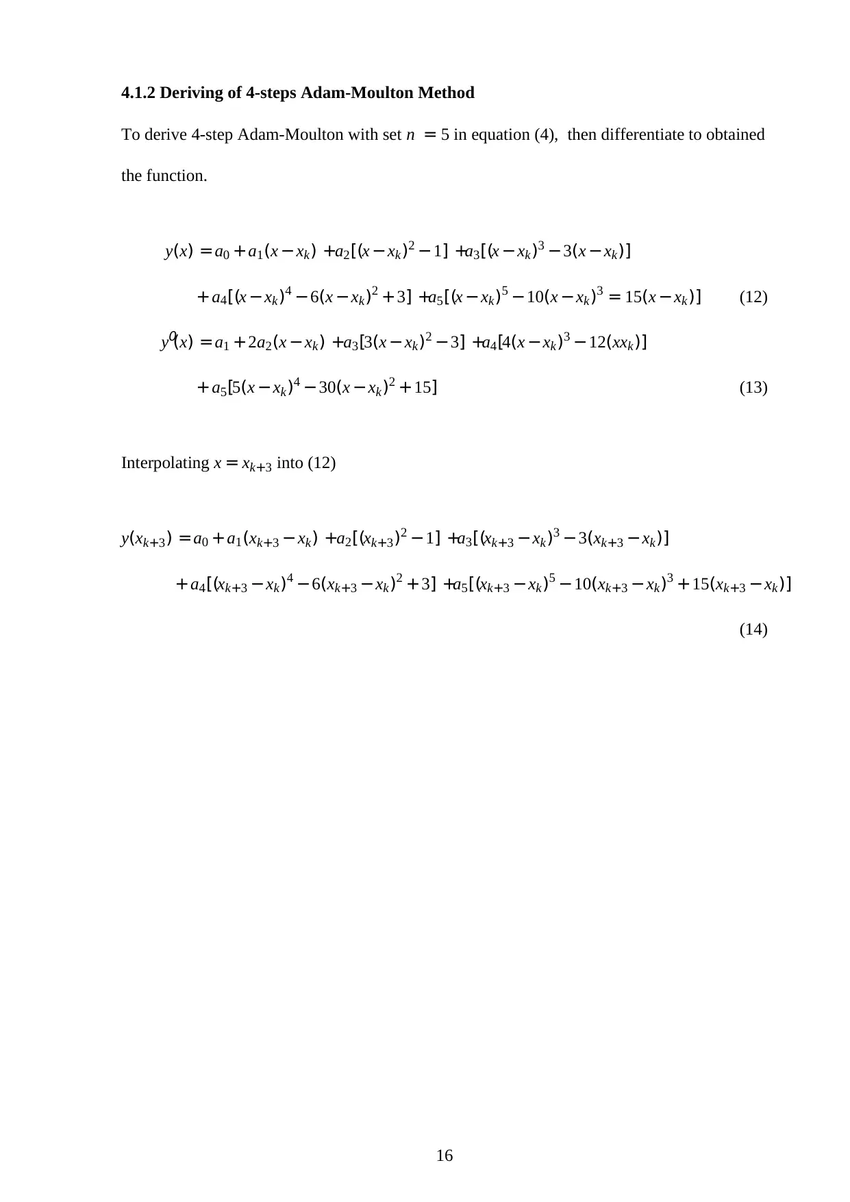
4.1.2 Deriving of 4-steps Adam-Moulton Method
To derive 4-step Adam-Moulton with set n = 5 in equation (4), then differentiate to obtained
the function.
y(x) =a0 +a1(x −xk) +a2[(x −xk)2 −1] +a3[(x −xk)3 −3(x −xk)]
+a4[(x −xk)4 −6(x −xk)2 +3] +a5[(x −xk)5 −10(x −xk)3 = 15(x −xk)] (12)
y0
(x) =a1 +2a2(x −xk) +a3[3(x −xk)2 −3] +a4[4(x −xk)3 −12(xxk)]
+a5[5(x −xk)4 −30(x −xk)2 +15] (13)
Interpolating x = xk+3 into (12)
y(xk+3) =a0 +a1(xk+3 −xk) +a2[(xk+3)2 −1] +a3[(xk+3 −xk)3 −3(xk+3 −xk)]
+a4[(xk+3 −xk)4 −6(xk+3 −xk)2 +3] +a5[(xk+3 −xk)5 −10(xk+3 −xk)3 +15(xk+3 −xk)]
(14)
16
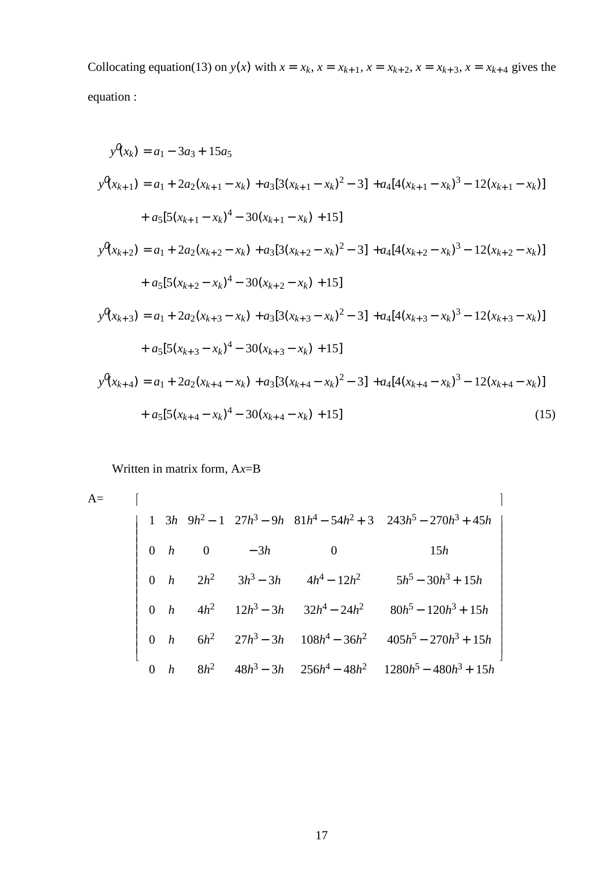
Collocating equation(13) on y(x) with x = xk, x = xk+1, x = xk+2, x = xk+3, x = xk+4 gives the
equation :
y0
(xk) =a1 −3a3 +15a5
y0
(xk+1) =a1 +2a2(xk+1 −xk) +a3[3(xk+1 −xk)2 −3] +a4[4(xk+1 −xk)3 −12(xk+1 −xk)]
+a5[5(xk+1 −xk)4 −30(xk+1 −xk) +15]
y0
(xk+2) =a1 +2a2(xk+2 −xk) +a3[3(xk+2 −xk)2 −3] +a4[4(xk+2 −xk)3 −12(xk+2 −xk)]
+a5[5(xk+2 −xk)4 −30(xk+2 −xk) +15]
y0
(xk+3) =a1 +2a2(xk+3 −xk) +a3[3(xk+3 −xk)2 −3] +a4[4(xk+3 −xk)3 −12(xk+3 −xk)]
+a5[5(xk+3 −xk)4 −30(xk+3 −xk) +15]
y0
(xk+4) =a1 +2a2(xk+4 −xk) +a3[3(xk+4 −xk)2 −3] +a4[4(xk+4 −xk)3 −12(xk+4 −xk)]
+a5[5(xk+4 −xk)4 −30(xk+4 −xk) +15] (15)
Written in matrix form, Ax=B
A=
1 3h 9h2 −1 27h3 −9h 81h4 −54h2 +3 243h5 −270h3 +45h
0 h 0 −3h 0 15h
0 h 2h2 3h3 −3h 4h4 −12h2 5h5 −30h3 +15h
0 h 4h2 12h3 −3h 32h4 −24h2 80h5 −120h3 +15h
0 h 6h2 27h3 −3h 108h4 −36h2 405h5 −270h3 +15h
0 h 8h2 48h3 −3h 256h4 −48h2 1280h5 −480h3 +15h
17
Paraphrase This Document
Need a fresh take? Get an instant paraphrase of this document with our AI Paraphraser
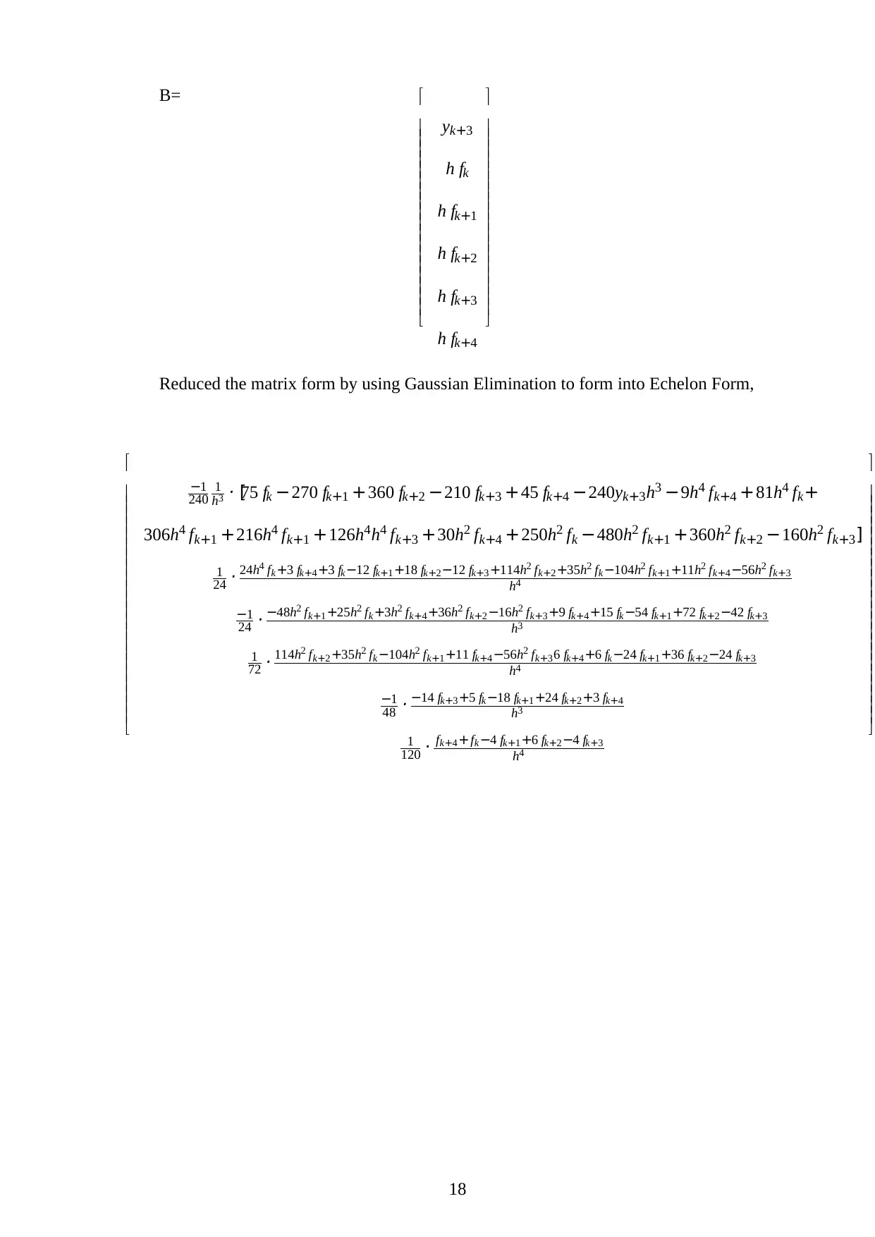
B=
yk+3
h fk
h fk+1
h fk+2
h fk+3
h fk+4
Reduced the matrix form by using Gaussian Elimination to form into Echelon Form,
−1
240 1
h3 · [75 fk −270 fk+1 +360 fk+2 −210 fk+3 +45 fk+4 −240yk+3h3 −9h4 fk+4 +81h4 fk+
306h4 fk+1 +216h4 fk+1 +126h4h4 fk+3 +30h2 fk+4 +250h2 fk −480h2 fk+1 +360h2 fk+2 −160h2 fk+3]
1
24 · 24h4 fk+3 fk+4+3 fk−12 fk+1+18 fk+2−12 fk+3+114h2 fk+2+35h2 fk−104h2 fk+1+11h2 fk+4−56h2 fk+3
h4
−1
24 · −48h2 fk+1+25h2 fk+3h2 fk+4+36h2 fk+2−16h2 fk+3+9 fk+4+15 fk −54 fk+1+72 fk+2−42 fk+3
h3
1
72 · 114h2 fk+2+35h2 fk−104h2 fk+1+11 fk+4−56h2 fk+36 fk+4+6 fk−24 fk+1+36 fk+2−24 fk+3
h4
−1
48 · −14 fk+3+5 fk−18 fk+1+24 fk+2+3 fk+4
h3
1
120 · fk+4+fk−4 fk+1+6 fk+2−4 fk+3
h4
18
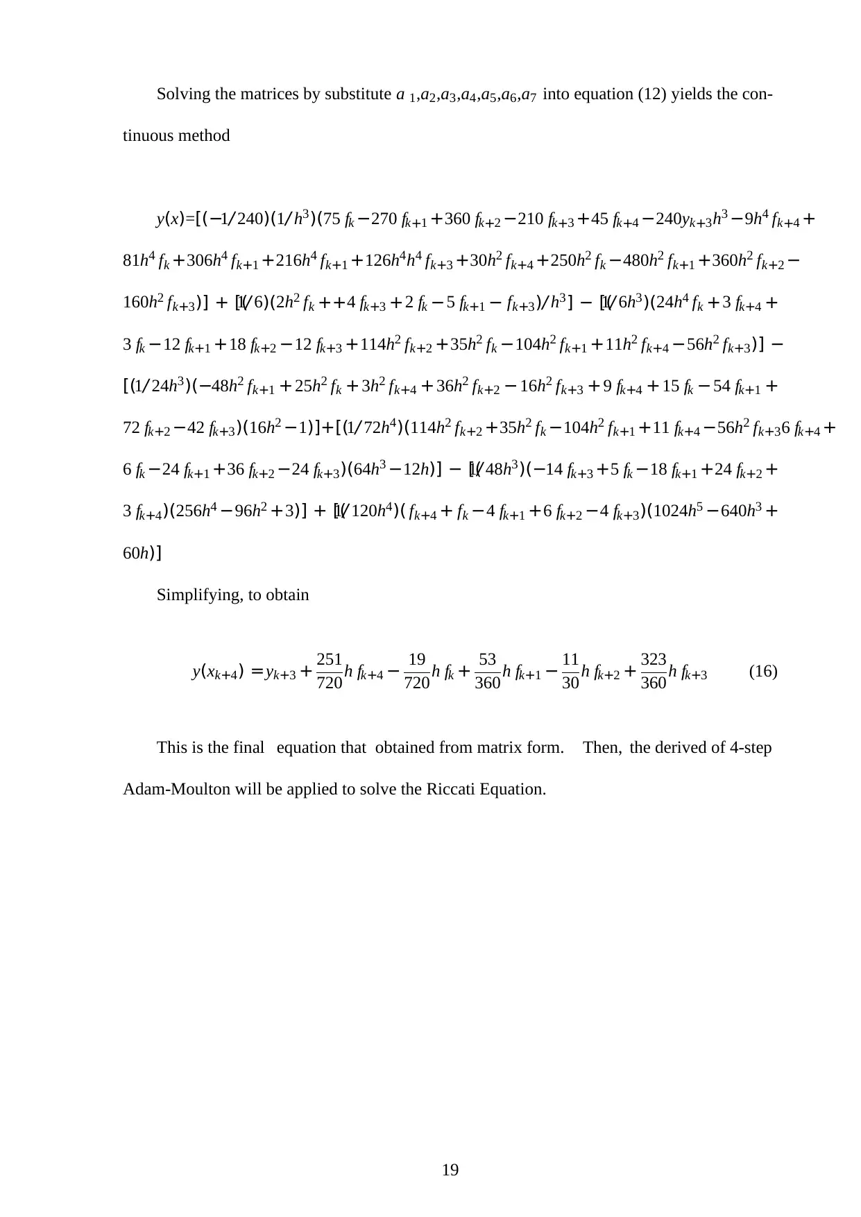
Solving the matrices by substitute a 1,a2,a3,a4,a5,a6,a7 into equation (12) yields the con-
tinuous method
y(x)=[(−1/ 240)(1/ h3)(75 fk −270 fk+1 +360 fk+2 −210 fk+3 +45 fk+4 −240yk+3h3 −9h4 fk+4 +
81h4 fk +306h4 fk+1 +216h4 fk+1 +126h4h4 fk+3 +30h2 fk+4 +250h2 fk −480h2 fk+1 +360h2 fk+2 −
160h2 fk+3)] + [(1/ 6)(2h2 fk ++4 fk+3 +2 fk −5 fk+1 − fk+3)/ h3] − [(1/ 6h3)(24h4 fk +3 fk+4 +
3 fk −12 fk+1 +18 fk+2 −12 fk+3 +114h2 fk+2 +35h2 fk −104h2 fk+1 +11h2 fk+4 −56h2 fk+3)] −
[(1/ 24h3)(−48h2 fk+1 +25h2 fk + 3h2 fk+4 + 36h2 fk+2 − 16h2 fk+3 + 9 fk+4 + 15 fk − 54 fk+1 +
72 fk+2 −42 fk+3)(16h2 −1)]+[(1/ 72h4)(114h2 fk+2 +35h2 fk −104h2 fk+1 +11 fk+4 −56h2 fk+36 fk+4 +
6 fk −24 fk+1 +36 fk+2 −24 fk+3)(64h3 −12h)] − [(1/ 48h3)(−14 fk+3 +5 fk −18 fk+1 +24 fk+2 +
3 fk+4)(256h4 −96h2 +3)] + [(1/ 120h4)( fk+4 + fk −4 fk+1 +6 fk+2 −4 fk+3)(1024h5 −640h3 +
60h)]
Simplifying, to obtain
y(xk+4) =yk+3 + 251
720h fk+4 − 19
720h fk + 53
360h fk+1 − 11
30h fk+2 + 323
360h fk+3 (16)
This is the final equation that obtained from matrix form. Then, the derived of 4-step
Adam-Moulton will be applied to solve the Riccati Equation.
19
4.2 Solving Riccati Equation
In order to solve the riccati equation, one equation has been taking from Ghomanjani & Khor-
ram (2017). Shown below is a riccati equation with initial value,
u0
(t) = −u(t) +u2(t),0 < t < 1
u(0) = 1
2 (17)
where the exact solution of above equation is
u(t) = e−t
1 +e−t (18)
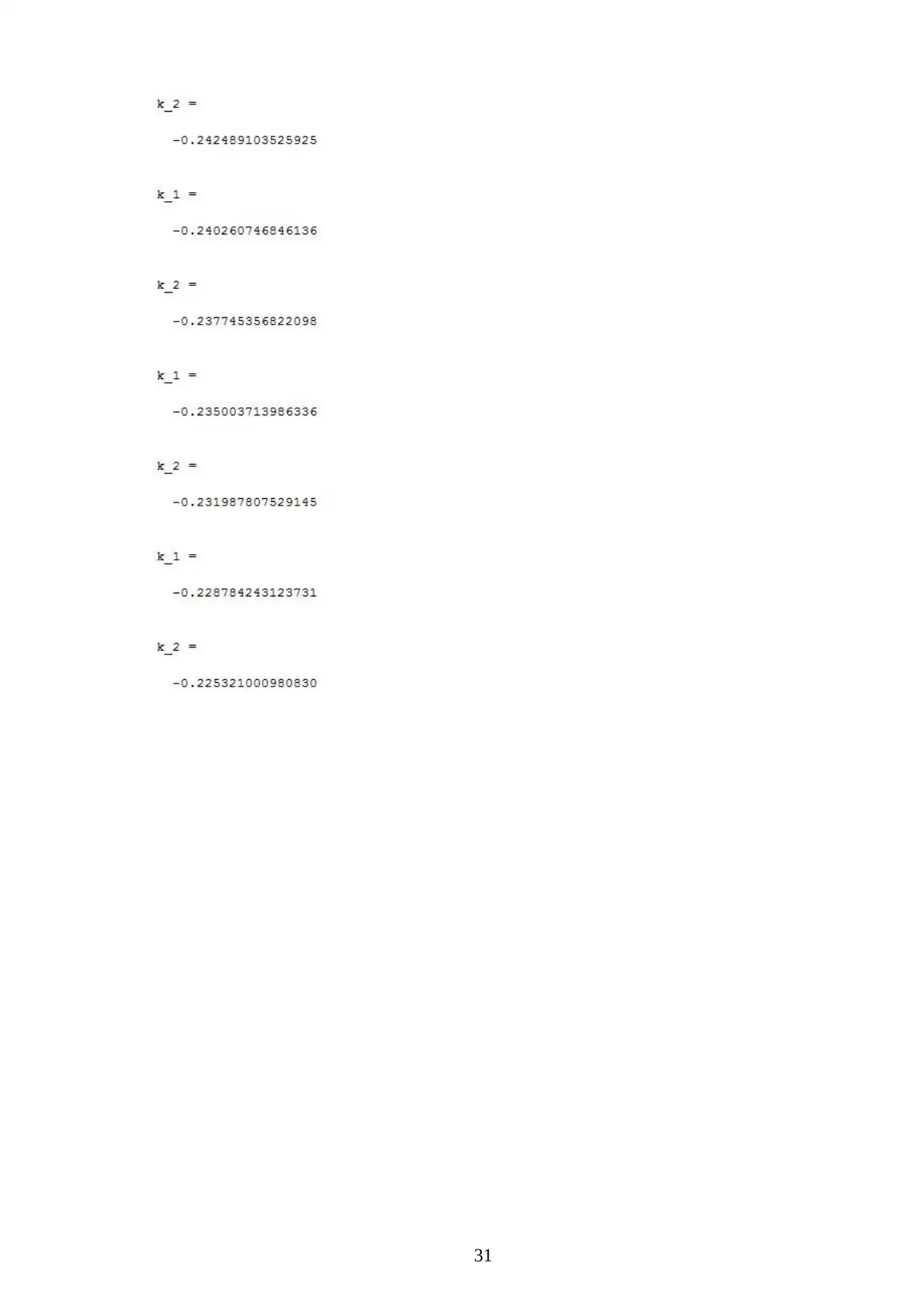
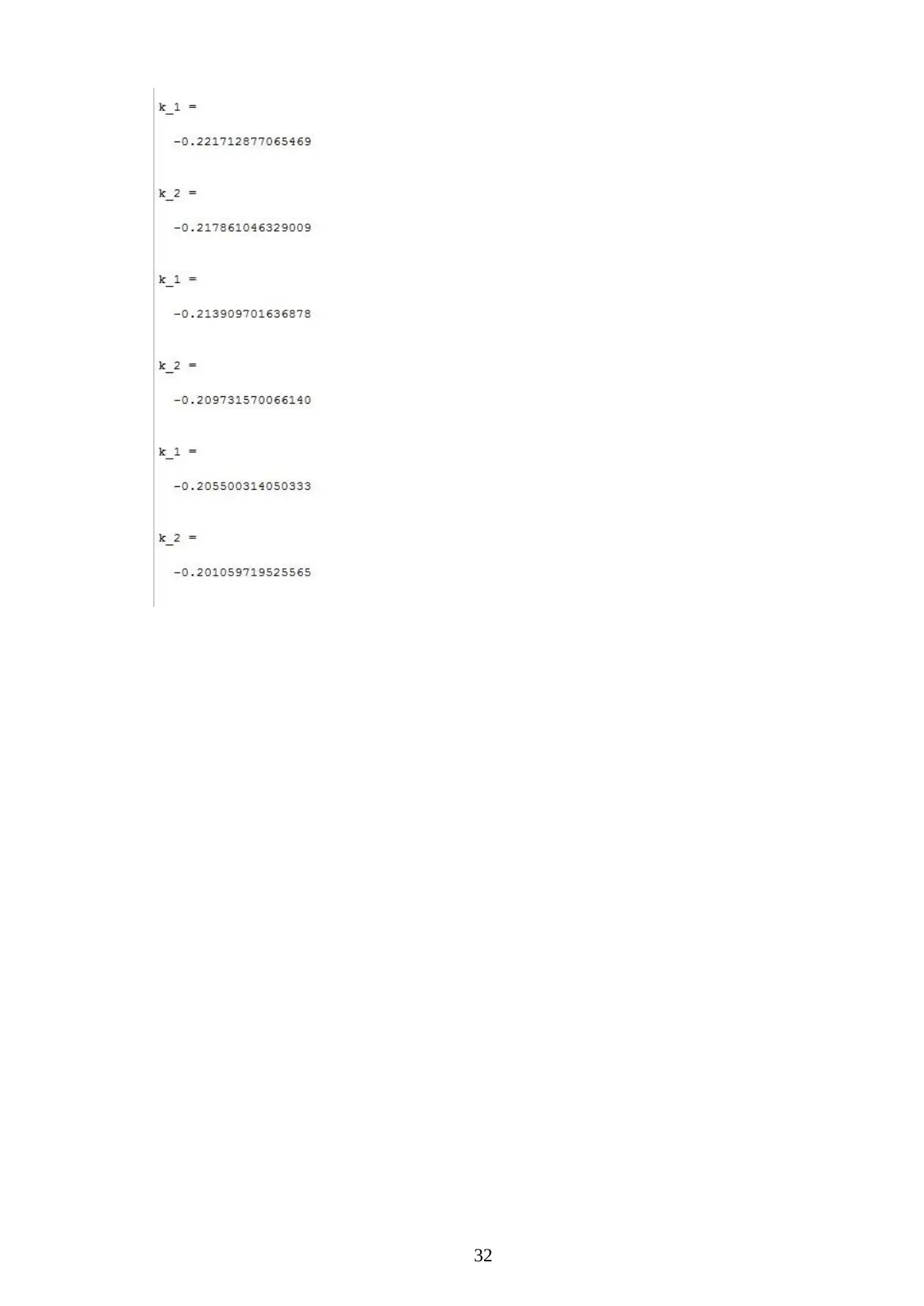
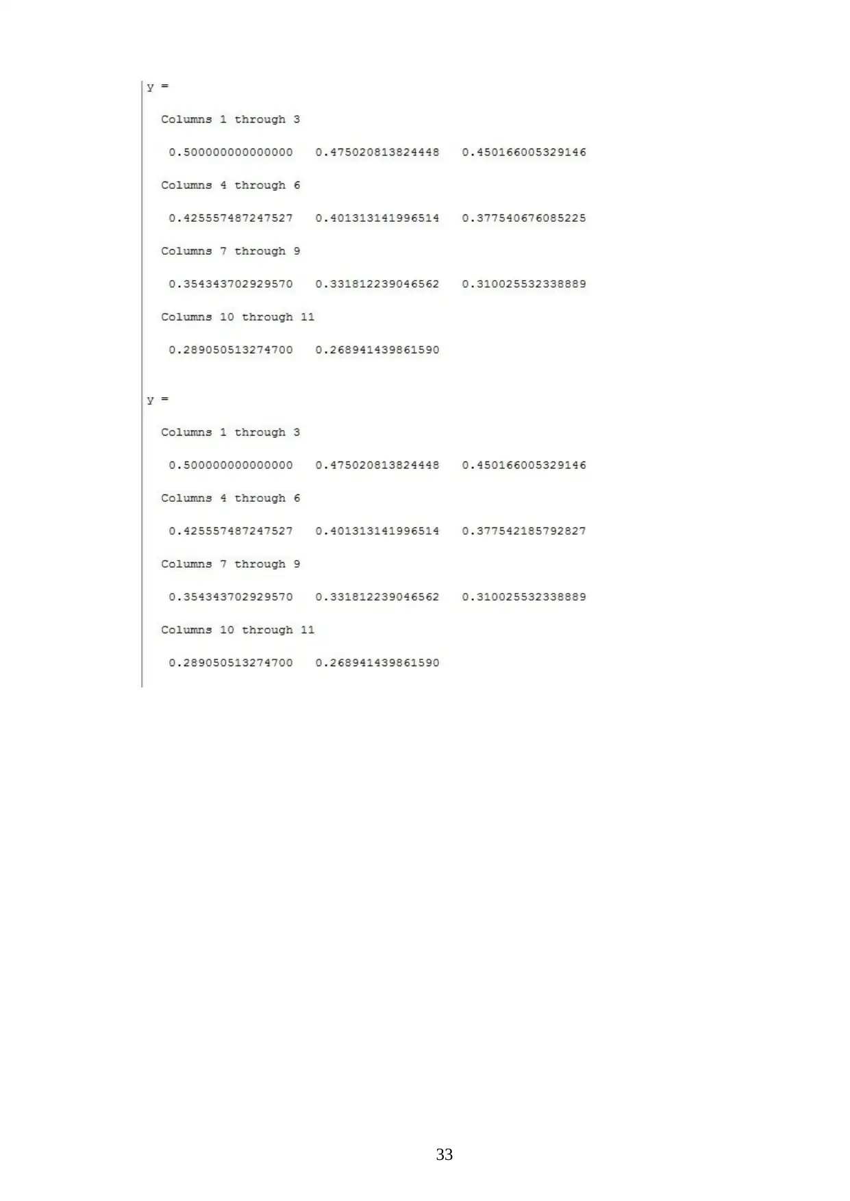
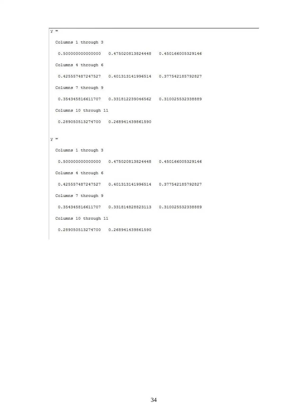
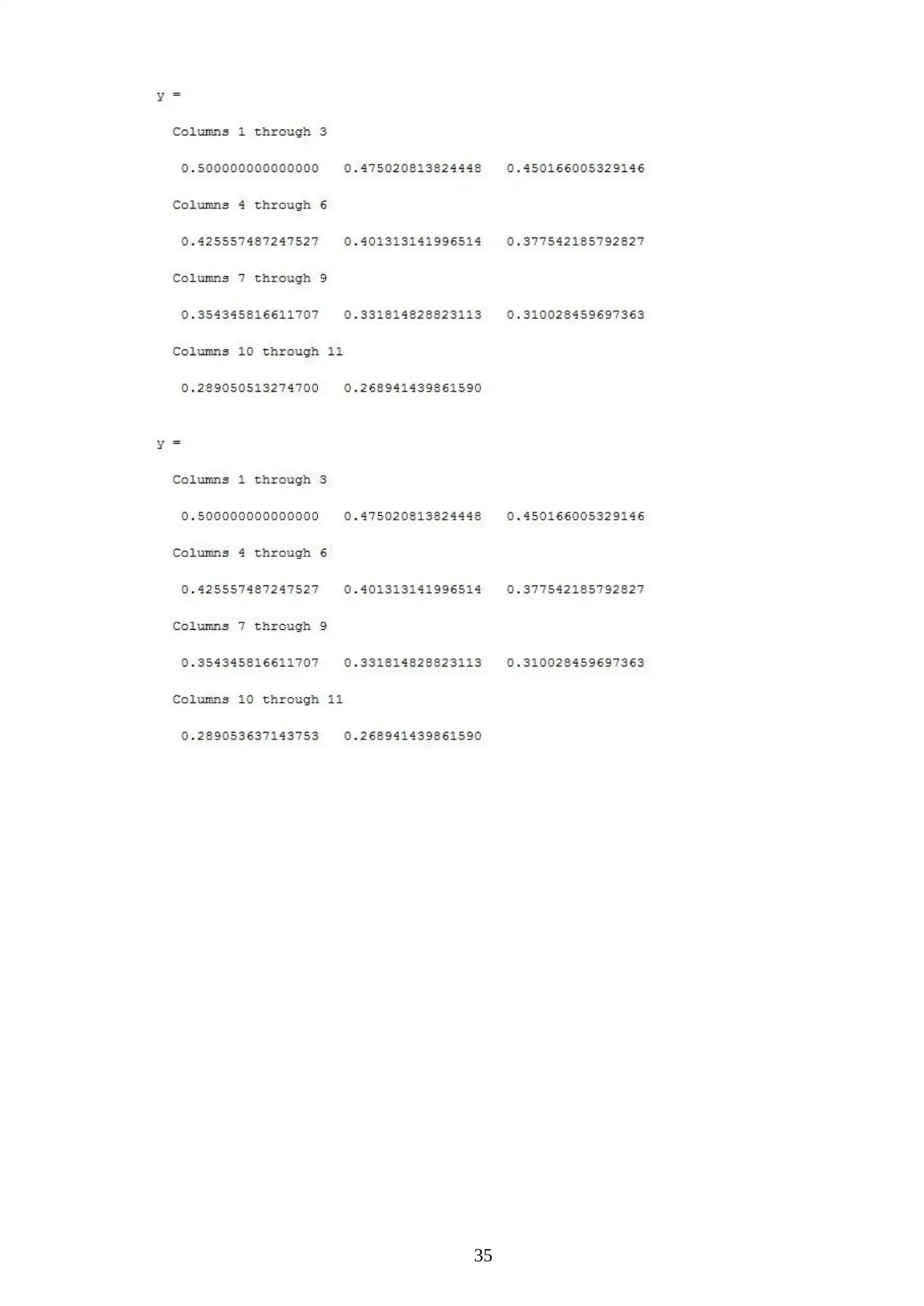
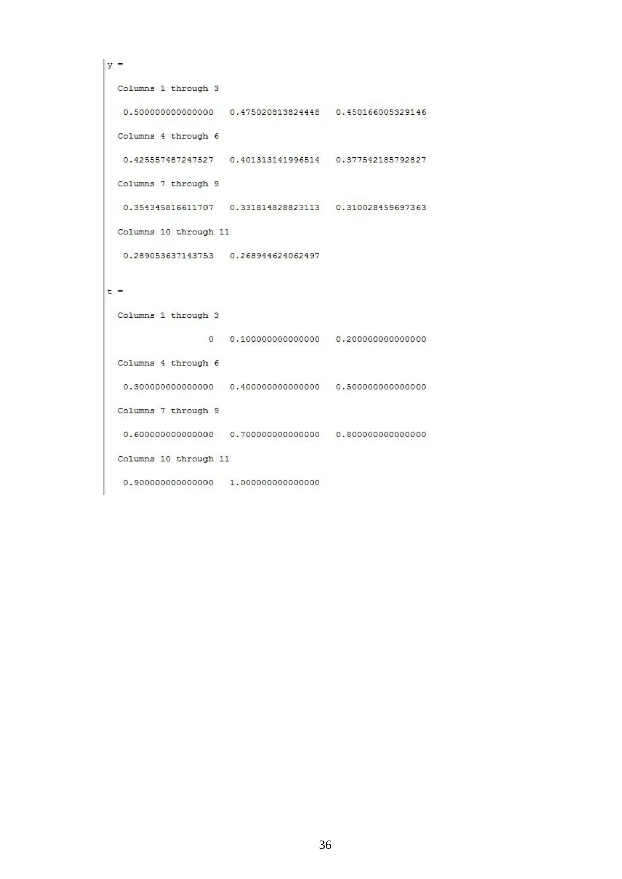
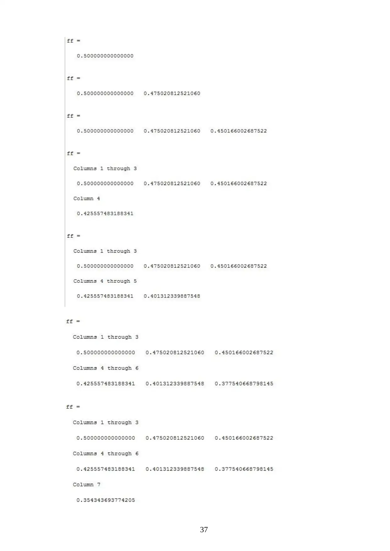
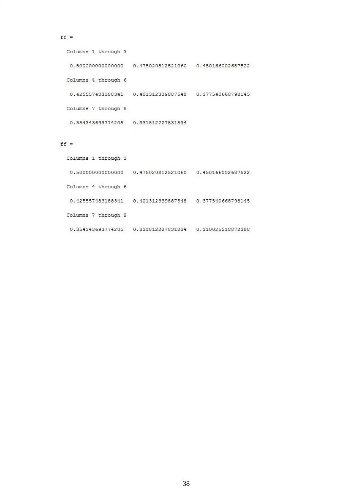
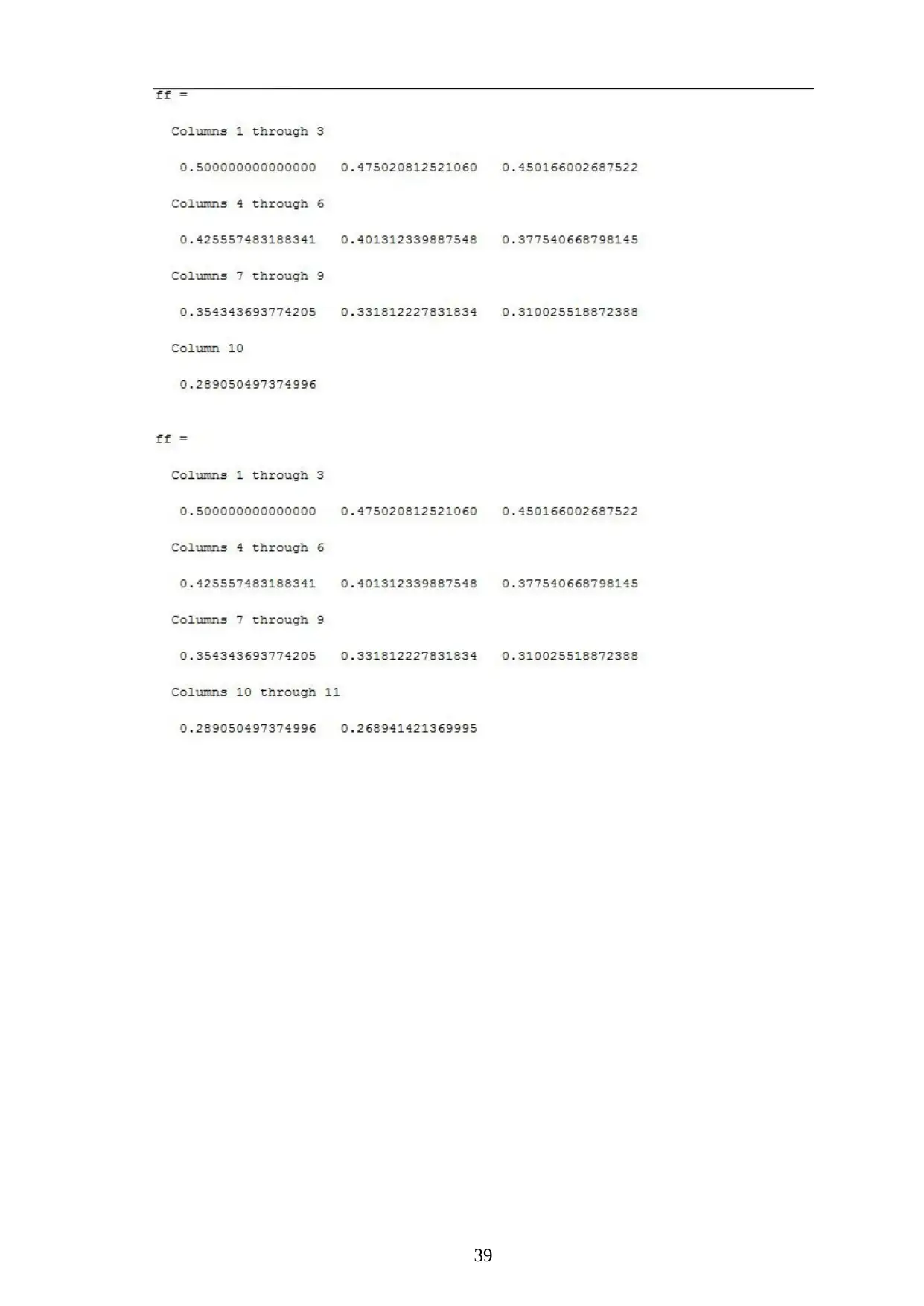
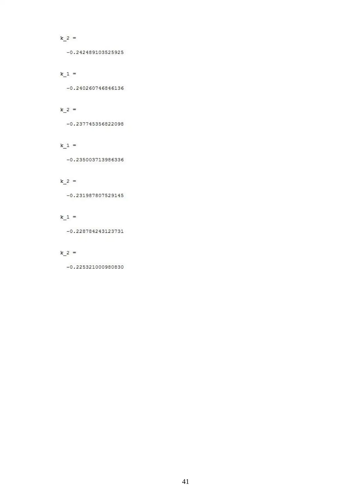
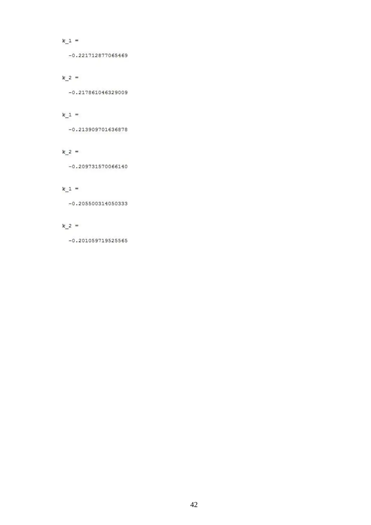
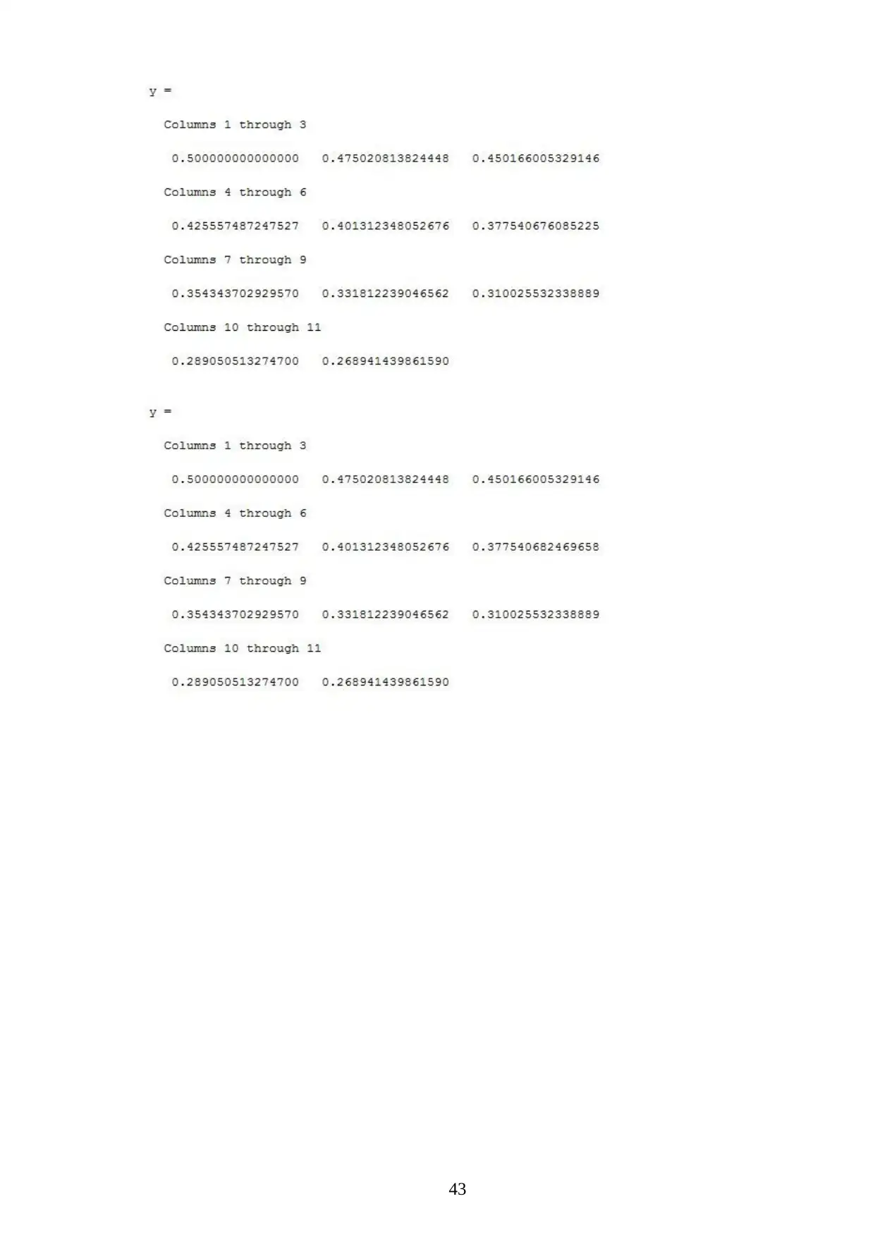
Solving Riccati Equation above by applying Adam Bashforth of discrete form in equation
(11) and Adam Moulton in equations (16) using MATLAB software are shown in figure 4.1 and
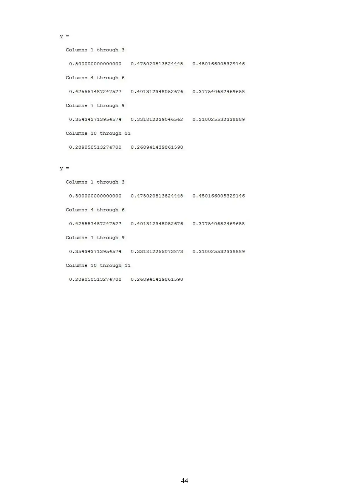
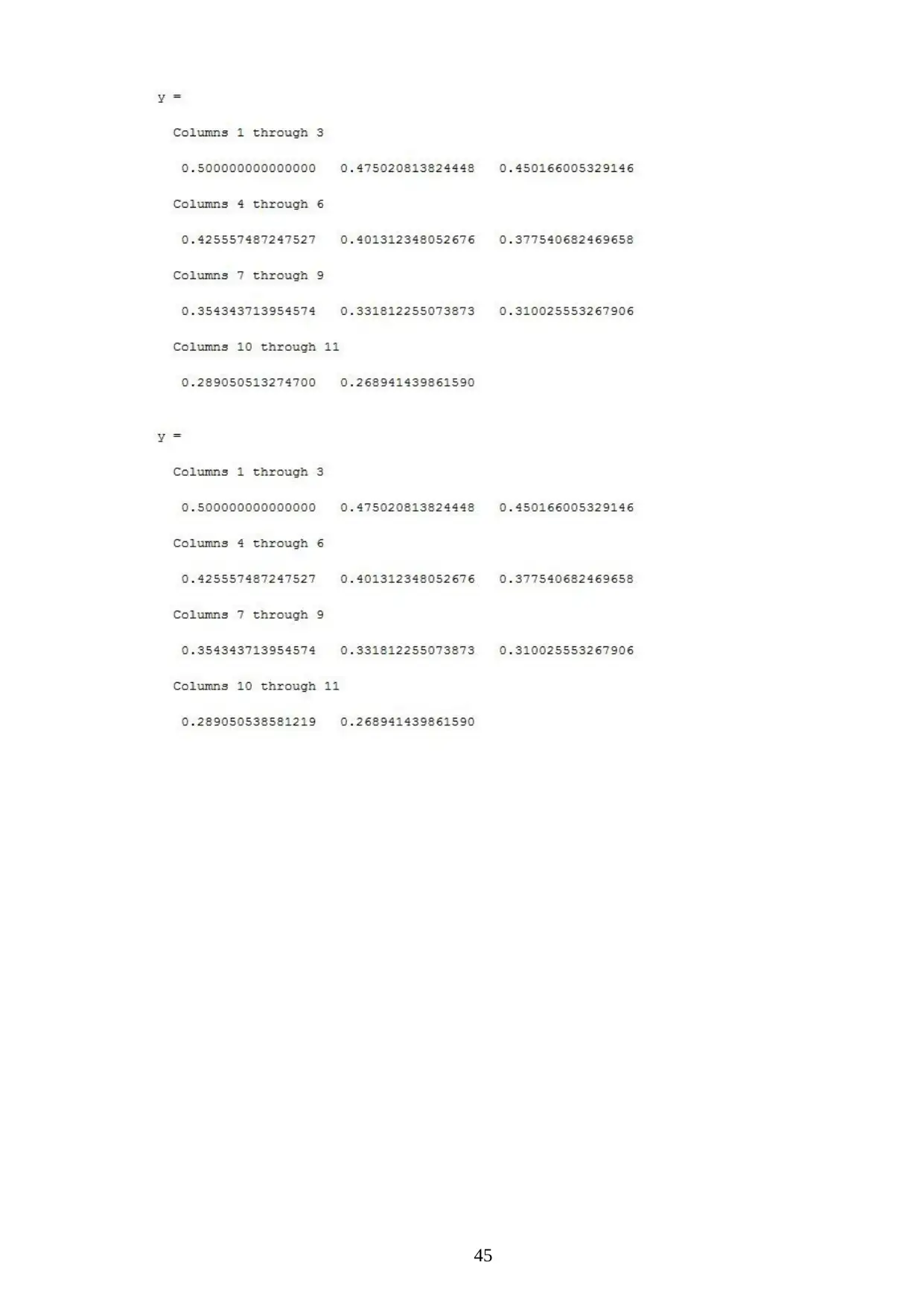
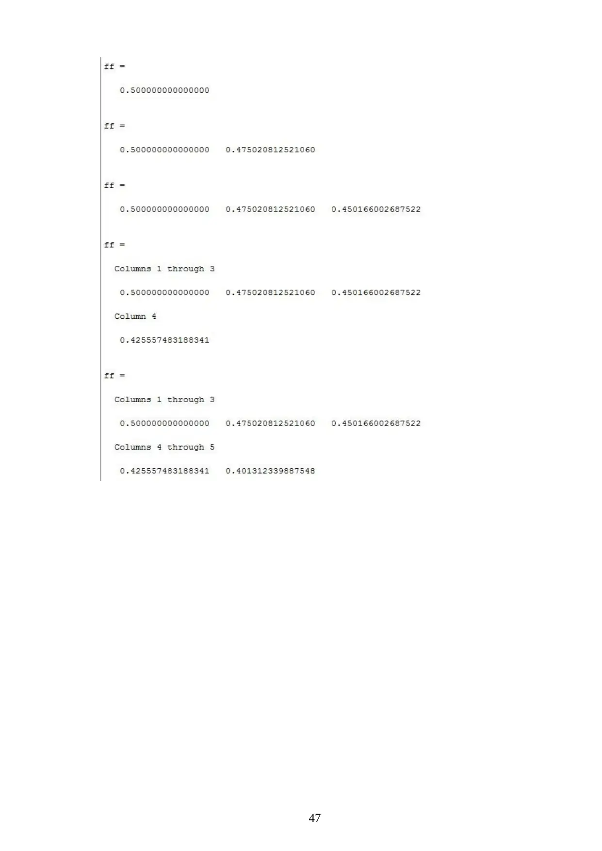
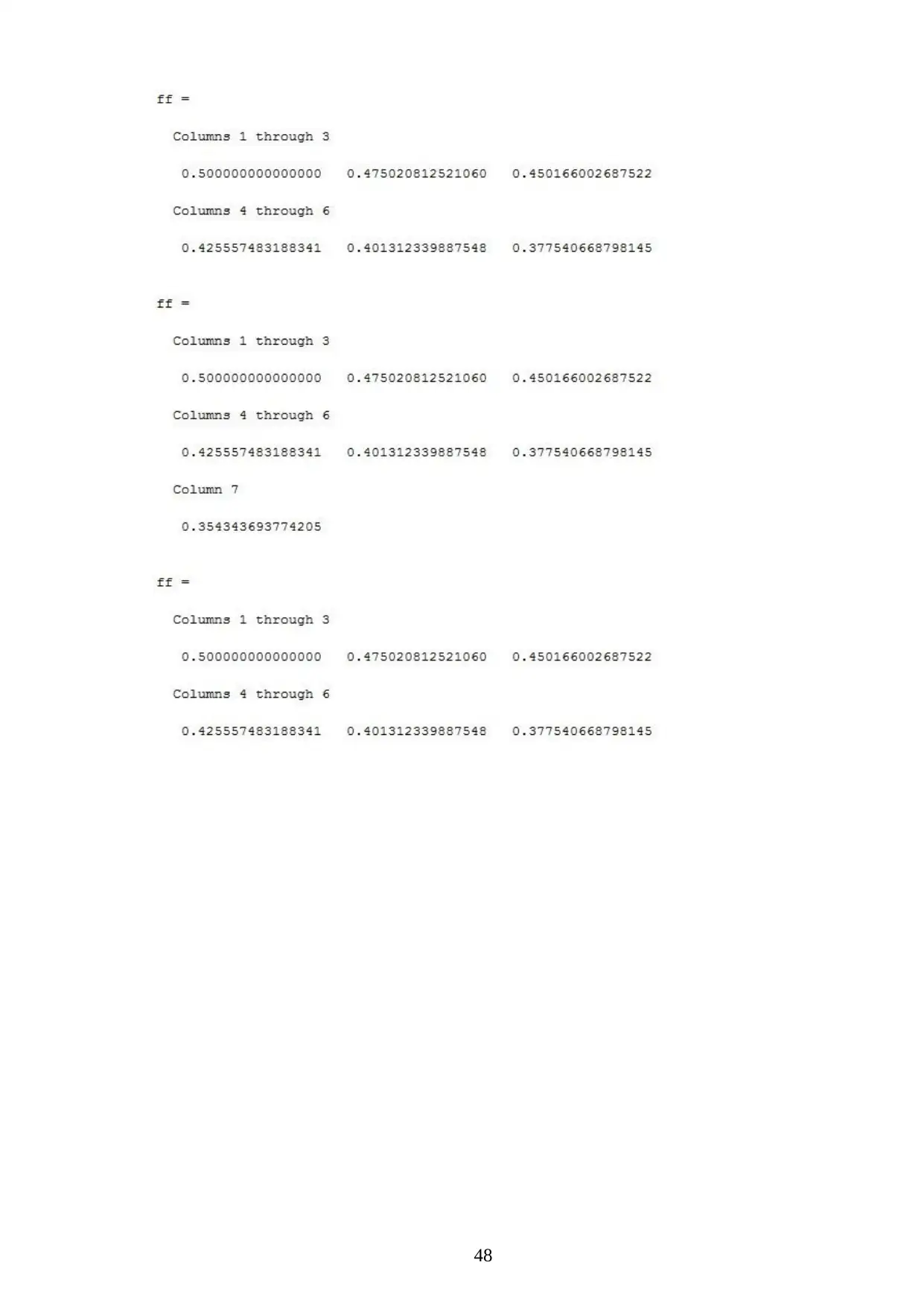
figure 4.2. All the result in MATLAB software are shown in Appendix A and Appendix B.
20
In order to solve the riccati equation, one equation has been taking from Ghomanjani & Khor-
ram (2017). Shown below is a riccati equation with initial value,
u0
(t) = −u(t) +u2(t),0 < t < 1
u(0) = 1
2 (17)
where the exact solution of above equation is
u(t) = e−t
1 +e−t (18)
Solving Riccati Equation above by applying Adam Bashforth of discrete form in equation
(11) and Adam Moulton in equations (16) using MATLAB software are shown in figure 4.1 and
figure 4.2. All the result in MATLAB software are shown in Appendix A and Appendix B.
20
Secure Best Marks with AI Grader
Need help grading? Try our AI Grader for instant feedback on your assignments.
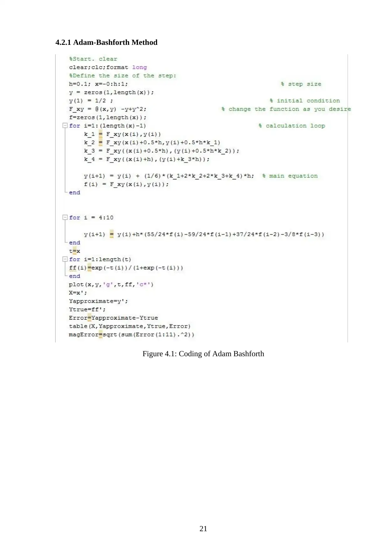
4.2.1 Adam-Bashforth Method
Figure 4.1: Coding of Adam Bashforth
21
Figure 4.1: Coding of Adam Bashforth
21
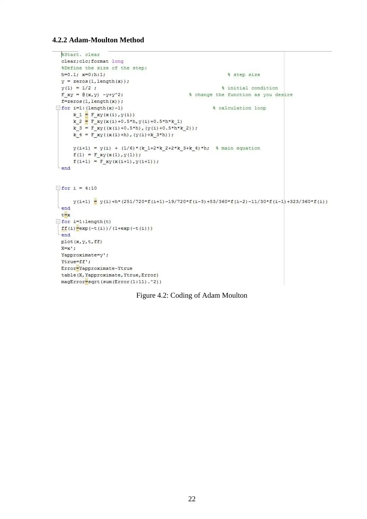
4.2.2 Adam-Moulton Method
Figure 4.2: Coding of Adam Moulton
22
Figure 4.2: Coding of Adam Moulton
22
4.3 Analysis of Results Obtained
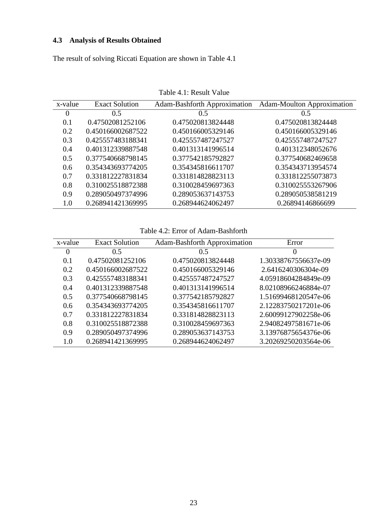
The result of solving Riccati Equation are shown in Table 4.1
Table 4.1: Result Value
x-value Exact Solution Adam-Bashforth Approximation Adam-Moulton Approximation
0 0.5 0.5 0.5
0.1 0.47502081252106 0.475020813824448 0.475020813824448
0.2 0.450166002687522 0.450166005329146 0.450166005329146
0.3 0.425557483188341 0.425557487247527 0.425557487247527
0.4 0.401312339887548 0.401313141996514 0.401312348052676
0.5 0.377540668798145 0.377542185792827 0.377540682469658
0.6 0.354343693774205 0.354345816611707 0.354343713954574
0.7 0.331812227831834 0.331814828823113 0.331812255073873
0.8 0.310025518872388 0.310028459697363 0.310025553267906
0.9 0.289050497374996 0.289053637143753 0.289050538581219
1.0 0.268941421369995 0.268944624062497 0.26894146866699
Table 4.2: Error of Adam-Bashforth
x-value Exact Solution Adam-Bashforth Approximation Error
0 0.5 0.5 0
0.1 0.47502081252106 0.475020813824448 1.30338767556637e-09
0.2 0.450166002687522 0.450166005329146 2.6416240306304e-09
0.3 0.425557483188341 0.425557487247527 4.05918604284849e-09
0.4 0.401312339887548 0.401313141996514 8.02108966246884e-07
0.5 0.377540668798145 0.377542185792827 1.51699468120547e-06
0.6 0.354343693774205 0.354345816611707 2.12283750217201e-06
0.7 0.331812227831834 0.331814828823113 2.60099127902258e-06
0.8 0.310025518872388 0.310028459697363 2.94082497581671e-06
0.9 0.289050497374996 0.289053637143753 3.13976875654376e-06
1.0 0.268941421369995 0.268944624062497 3.20269250203564e-06
23
Paraphrase This Document
Need a fresh take? Get an instant paraphrase of this document with our AI Paraphraser
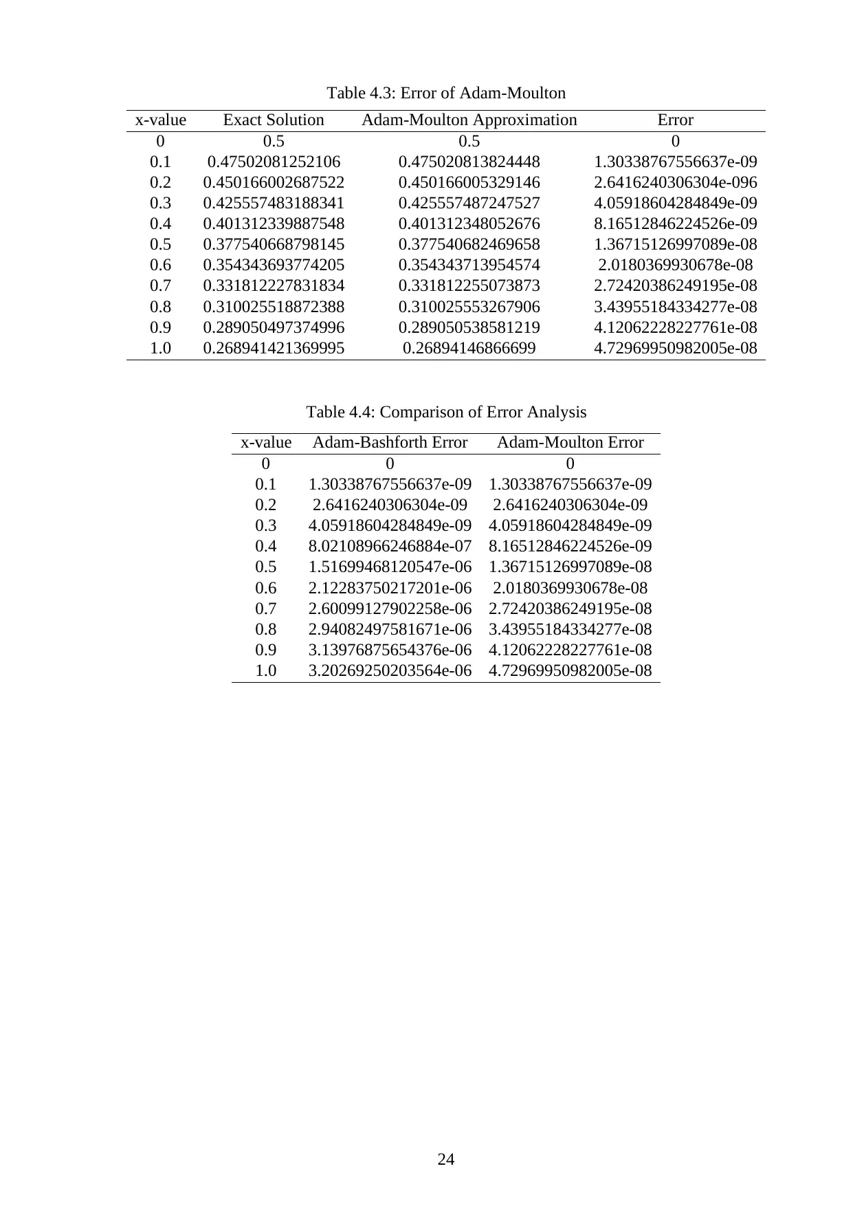
Table 4.3: Error of Adam-Moulton
x-value Exact Solution Adam-Moulton Approximation Error
0 0.5 0.5 0
0.1 0.47502081252106 0.475020813824448 1.30338767556637e-09
0.2 0.450166002687522 0.450166005329146 2.6416240306304e-096
0.3 0.425557483188341 0.425557487247527 4.05918604284849e-09
0.4 0.401312339887548 0.401312348052676 8.16512846224526e-09
0.5 0.377540668798145 0.377540682469658 1.36715126997089e-08
0.6 0.354343693774205 0.354343713954574 2.0180369930678e-08
0.7 0.331812227831834 0.331812255073873 2.72420386249195e-08
0.8 0.310025518872388 0.310025553267906 3.43955184334277e-08
0.9 0.289050497374996 0.289050538581219 4.12062228227761e-08
1.0 0.268941421369995 0.26894146866699 4.72969950982005e-08
Table 4.4: Comparison of Error Analysis
x-value Adam-Bashforth Error Adam-Moulton Error
0 0 0
0.1 1.30338767556637e-09 1.30338767556637e-09
0.2 2.6416240306304e-09 2.6416240306304e-09
0.3 4.05918604284849e-09 4.05918604284849e-09
0.4 8.02108966246884e-07 8.16512846224526e-09
0.5 1.51699468120547e-06 1.36715126997089e-08
0.6 2.12283750217201e-06 2.0180369930678e-08
0.7 2.60099127902258e-06 2.72420386249195e-08
0.8 2.94082497581671e-06 3.43955184334277e-08
0.9 3.13976875654376e-06 4.12062228227761e-08
1.0 3.20269250203564e-06 4.72969950982005e-08
24
5 RESULTS AND DISCUSSION
In this section, all the result obtained from the calculation are presented. This part contained the
explanation and elaboration of the obtained result. The interpretation of the formula has been
shown in implementation section.
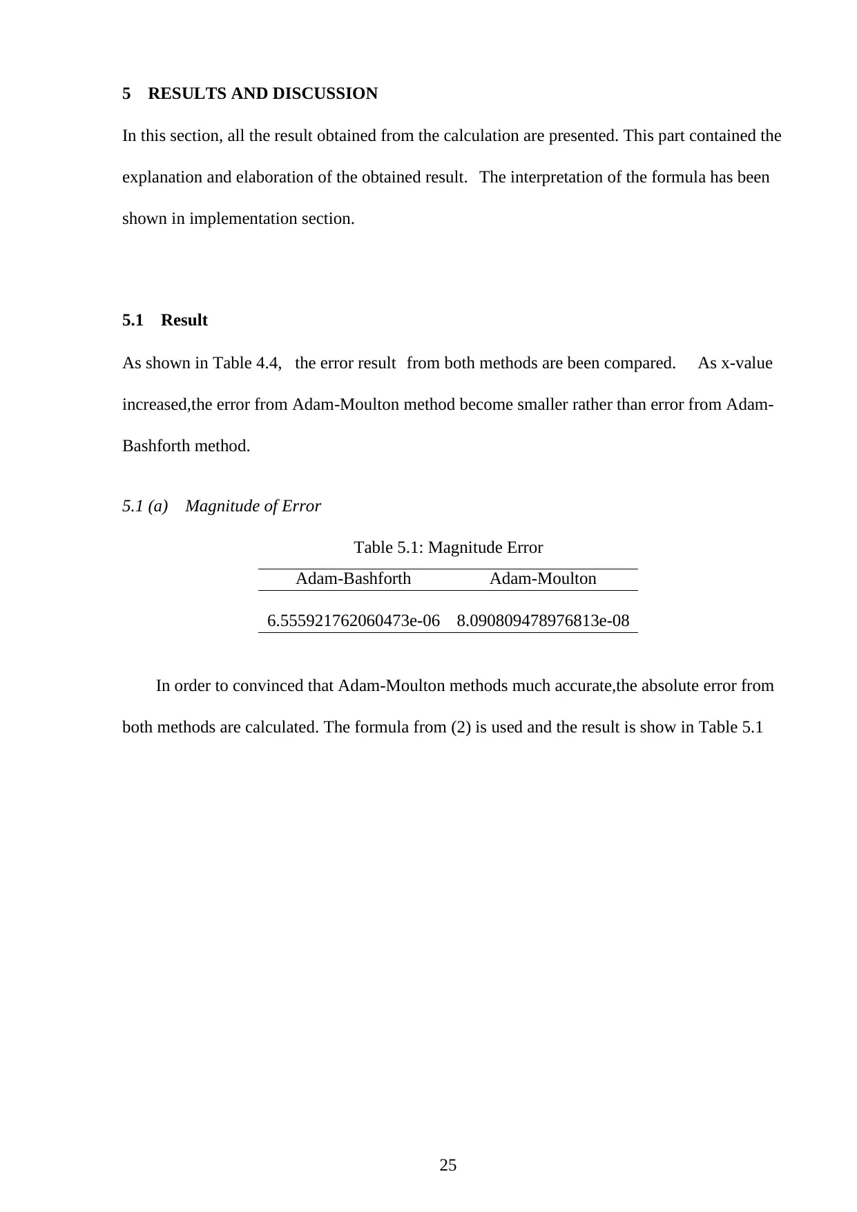
5.1 Result
As shown in Table 4.4, the error result from both methods are been compared. As x-value
increased,the error from Adam-Moulton method become smaller rather than error from Adam-
Bashforth method.
5.1 (a) Magnitude of Error
Table 5.1: Magnitude Error
Adam-Bashforth Adam-Moulton
6.555921762060473e-06 8.090809478976813e-08
In order to convinced that Adam-Moulton methods much accurate,the absolute error from
both methods are calculated. The formula from (2) is used and the result is show in Table 5.1
25
In this section, all the result obtained from the calculation are presented. This part contained the
explanation and elaboration of the obtained result. The interpretation of the formula has been
shown in implementation section.
5.1 Result
As shown in Table 4.4, the error result from both methods are been compared. As x-value
increased,the error from Adam-Moulton method become smaller rather than error from Adam-
Bashforth method.
5.1 (a) Magnitude of Error
Table 5.1: Magnitude Error
Adam-Bashforth Adam-Moulton
6.555921762060473e-06 8.090809478976813e-08
In order to convinced that Adam-Moulton methods much accurate,the absolute error from
both methods are calculated. The formula from (2) is used and the result is show in Table 5.1
25
5.2 Discussion
After the result obtained, it show that approximation of Adam-Moulton on Riccati equation is
much smaller than Adam-Bashforth. The accuracy of analysis is discuss from the result show
that Adam-Moulton is more accurate than Adam-Bashforth. As my opinion, the Riccati Equa-
tion is an example of non-linear differential equation that can be solve using Adam-Bashforth
and Moulton methods. Regarding the result, both Adam-Bashforth and Moulton only can be
used in first order of differential equation. Thus, it is relevant to approximate Riccati Equation
using both methods and compare with analytical result.
Advantages of this methods is stable even if small changes in the initial condition result
in only small changes in the computed solution. Moreover this method requires only one new
function evaluation for each step. It will lead to great savings in time. Disadvantages of this
method is that it require four function evaluation from RK4 method to solve. It means that this
method is depend on the other method.
26
Secure Best Marks with AI Grader
Need help grading? Try our AI Grader for instant feedback on your assignments.
6 CONCLUSIONS AND RECOMMENDATIONS
In this study, Adam-Bashforth and Adam-Moulton methods was applied to solve Riccati equa-
tion. Both method was derived to get 4-step for Adam-Bashforth and Adam-Moulton using
manual calculation and continue using Maple software. Hence both methods are used to solve
nonlinear differential equation such as Riccati equation. The Riccati equation are obtained
from Ghomanjani & Khorram (2017) to help in solving using Adam-Bashforth and Adam-
Moulton methods. After that, the accuracy of both Adam methods on the Riccati equation were
analysed. From this analysis, Adam-Bashforth method was found to be more accurate than
Adam-Bashforth methods.
After finish this study, there are many numerical methods been used to solve any differ-
ential equation. In future, these methods can be explore whether suitable to used on any other
non-linear differential equation.
27
REFERENCES
Aboiyar, T., Luga, T., & Iyorter, B. (2015). Derivation of Continuous Linear Multistep Methods
Using Hermite Polynomials as Basis Functions. American Journal of Applied Mathematics
and Statistics, 3(6), 220–225. Retrieved from http://pubs.sciepub.com/ajams/3/6/2
Amman, H. M., & Neudecker, H. (1997). Numerical Solutions Of The Algebraic Matrix Riccati
Equation. Journal of Economic Dynamics and Control, 21(8), 363–369.
Anake, B., & Ashibel Cugp, T. (2011). Continuous Implicit Hybrid One-Step Methods For The
Solution of Initial Value Problems of General Second-Order Ordinary Differential Equations.
Natural and Applied Sciences, 1(4), 157–170.
Areo, E. A., & Adeniyi, R. B. (2013). Self-Starting Linear Multistep Method For Direct Solu-
tion of Initial Value Problems of Second Order Ordinary Differential Equations. International
Journal of Pure and Applied Mathematics, 82(3), 345–364.
Awoyemi, D. (1999). A class of continuous methods for general second order initial value
problems in ordinary differential equations. International Journal of Computer Mathemat-
ics,, 72(1), 29–37.
Butcher, J. C. (2000). Numerical Methods for Ordinary Diferential Equations in the 20th
Century. Journal of Computational and Applied Mathematics, 125(5), 1–29. Retrieved from
www.elsevier.nl/locate/cam
C Butcher John, B. J. (1987). The Numerical Analysis of Ordinary Differential Equations:
Runge-Kutta and General Linear Methods. A Wiley Interscience, 7(15), 5–12.
Chiou, J. C., & Wu, S. D. (1999). On the Generation of Higher Order Numerical Integration
Methods Using Lower Order Adams-Bashforth and Adams-Moulton Methods. Journal of
Computational and Applied Mathematics, 5(9), 19–29.
28
File, G., & Aga, T. (2016). Numerical Solution Of Quadratic Riccati Differential Equations.
Journal of Basic and Applied Science 3, 3(11), 392–397.
Garrappa, R. (2009). On some explicit Adams multistep methods for fractional differential
equations. Journal of Computational and Applied Mathematics, 3(4), 30–35.
Ghomanjani, F., & Khorram, E. (2017). Approximate Solution For Quadratic Riccati Differen-
tial Equation. Journal of Taibah University for Science, 11(9), 246–250.
Jator, S. (2001). Improvement in Adam-Moulton Method for FIrst Order Initial Value Problems.
Journal Of Tennese Academy Of Science, 76(2), 57–60.
Misirli, E., & Gurefe, Y. (2011). Multiplicative Adams Bashforth–Moulton methods. Numer
Algor, 57(3), 425–439.
Petzoldf, L. R. (1986). Order Results For Implicit Runge-Kutta Methods Applied To Differen-
tial/Algebraic System. Siam J. Numerical Analysis, 23(4), 1–16.
29
Paraphrase This Document
Need a fresh take? Get an instant paraphrase of this document with our AI Paraphraser
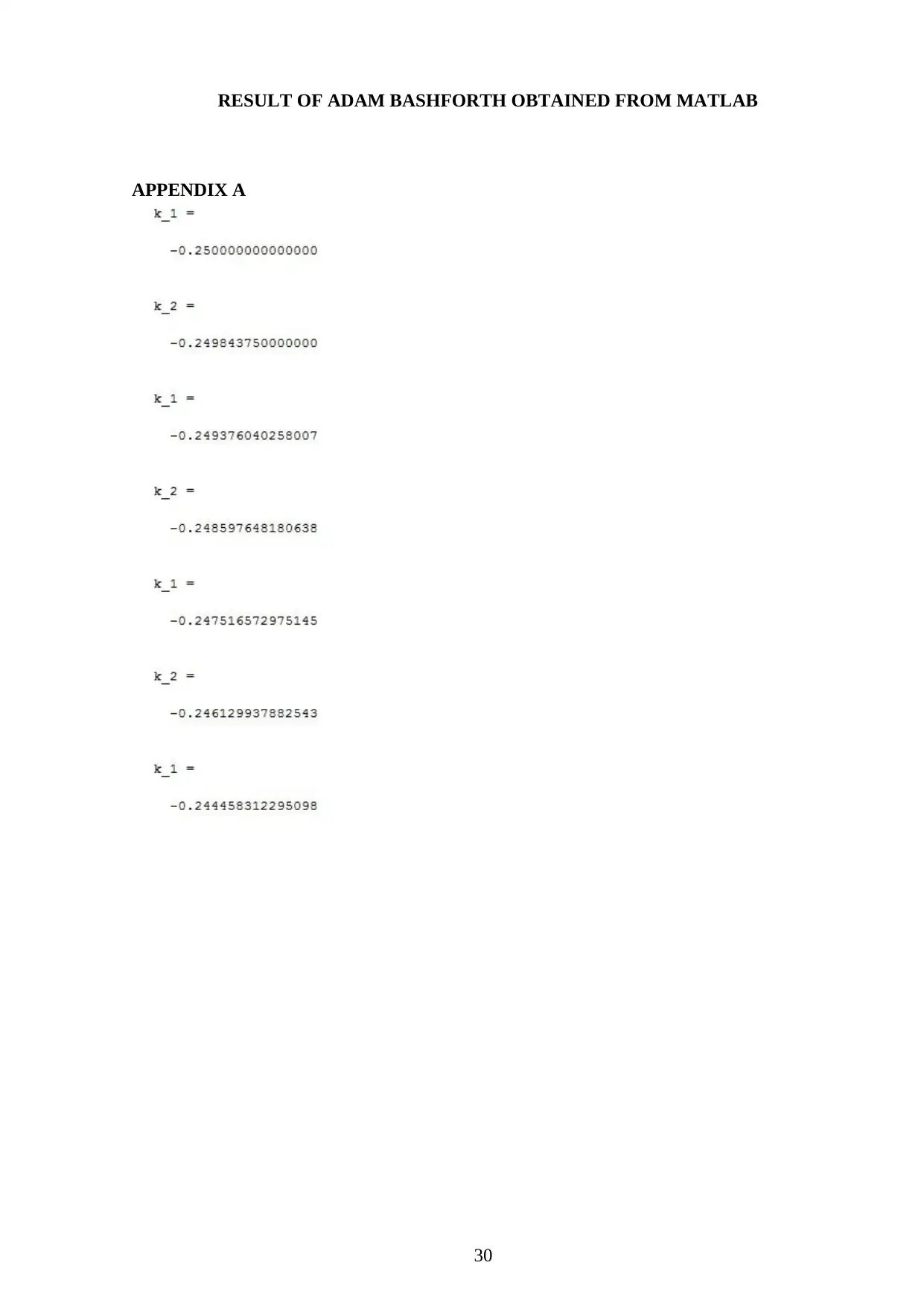
RESULT OF ADAM BASHFORTH OBTAINED FROM MATLAB
APPENDIX A
30
APPENDIX A
30
31
32
Secure Best Marks with AI Grader
Need help grading? Try our AI Grader for instant feedback on your assignments.
33
34
35
Paraphrase This Document
Need a fresh take? Get an instant paraphrase of this document with our AI Paraphraser
36
37
38
Secure Best Marks with AI Grader
Need help grading? Try our AI Grader for instant feedback on your assignments.
39

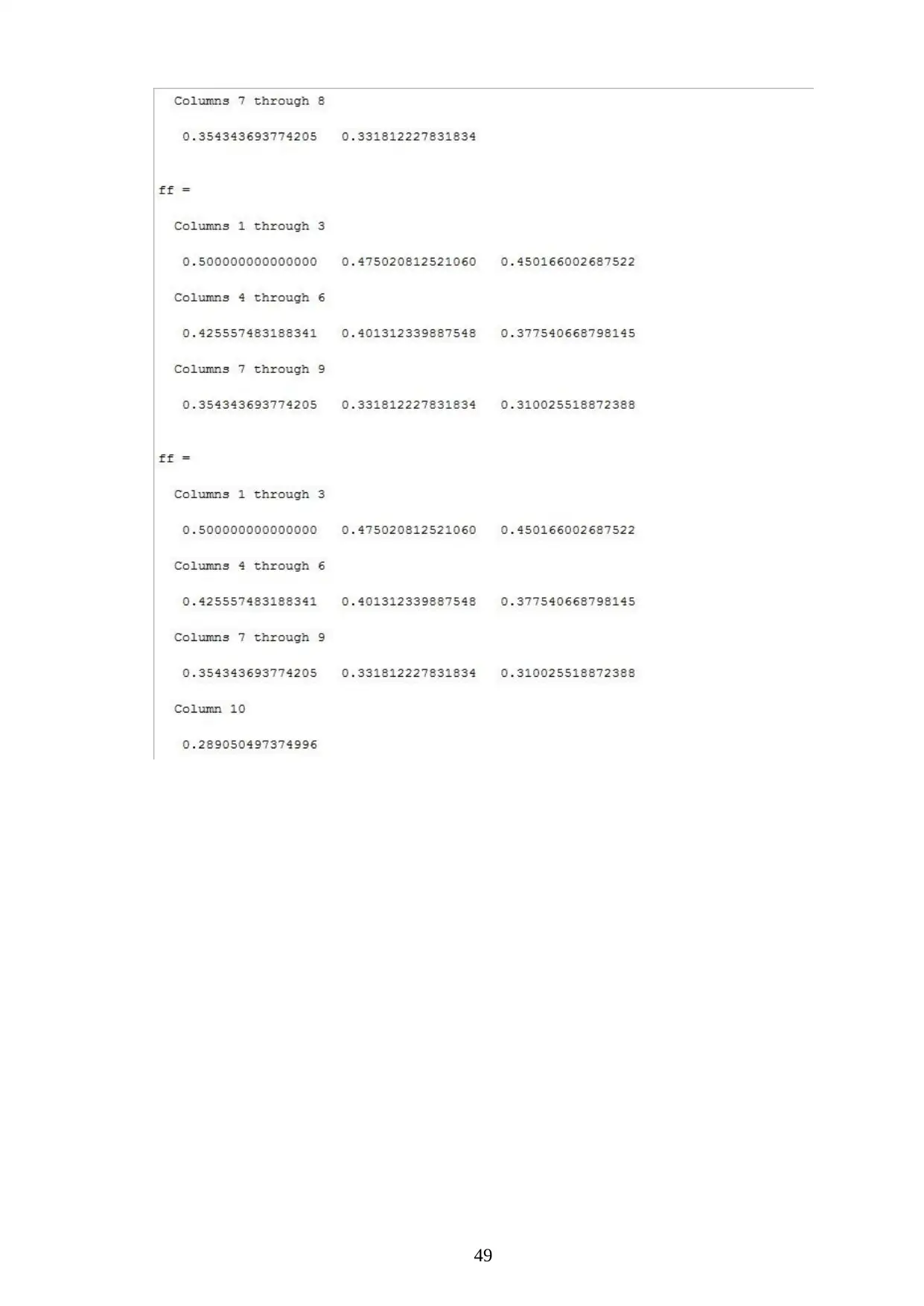
RESULT OF ADAM MOULTON OBTAINED FROM MATLAB
APPENDIX B
40
APPENDIX B
40
41
Paraphrase This Document
Need a fresh take? Get an instant paraphrase of this document with our AI Paraphraser
42
43
44
Secure Best Marks with AI Grader
Need help grading? Try our AI Grader for instant feedback on your assignments.
45

46
47
Paraphrase This Document
Need a fresh take? Get an instant paraphrase of this document with our AI Paraphraser
48
49
1 out of 57


Your All-in-One AI-Powered Toolkit for Academic Success.
+13062052269
info@desklib.com
Available 24*7 on WhatsApp / Email
![[object Object]](/_next/static/media/star-bottom.7253800d.svg)
Unlock your academic potential
© 2024 | Zucol Services PVT LTD | All rights reserved.