Linear Programming Solutions and Analysis
VerifiedAdded on 2020/02/24
|26
|3869
|850
AI Summary
The assignment focuses on applying linear programming techniques to solve a real-world business problem. Students are tasked with finding the optimal production mix for a company manufacturing printers and keyboards to maximize contribution margin. The solution process involves graphically representing the feasible region, identifying corner points, and evaluating the objective function at each point to determine the optimal solution.
Contribute Materials
Your contribution can guide someone’s learning journey. Share your
documents today.
BF360 - Operations Research Assignment One (July 2017)
Name of the student
Name of the University
Author Note
Name of the student
Name of the University
Author Note
Secure Best Marks with AI Grader
Need help grading? Try our AI Grader for instant feedback on your assignments.
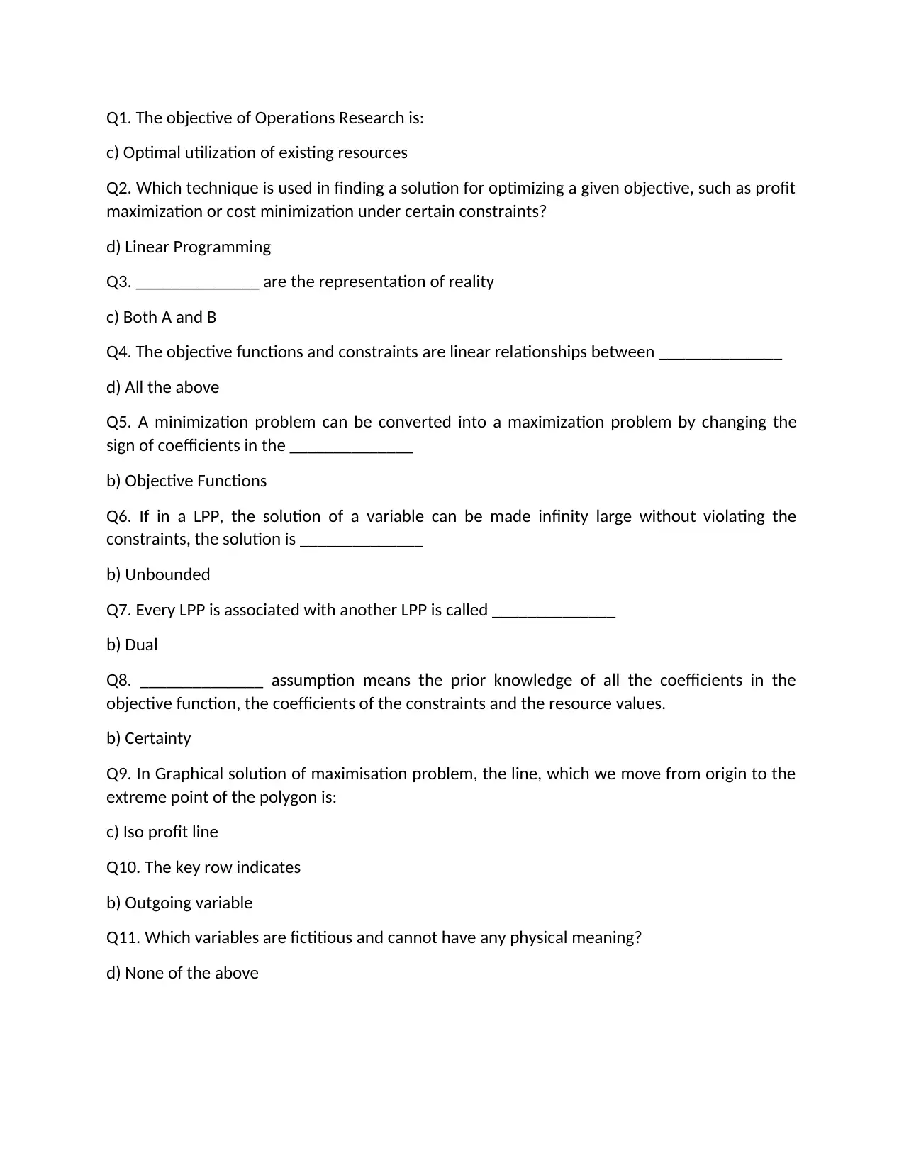
Q1. The objective of Operations Research is:
c) Optimal utilization of existing resources
Q2. Which technique is used in finding a solution for optimizing a given objective, such as profit
maximization or cost minimization under certain constraints?
d) Linear Programming
Q3. ______________ are the representation of reality
c) Both A and B
Q4. The objective functions and constraints are linear relationships between ______________
d) All the above
Q5. A minimization problem can be converted into a maximization problem by changing the
sign of coefficients in the ______________
b) Objective Functions
Q6. If in a LPP, the solution of a variable can be made infinity large without violating the
constraints, the solution is ______________
b) Unbounded
Q7. Every LPP is associated with another LPP is called ______________
b) Dual
Q8. ______________ assumption means the prior knowledge of all the coefficients in the
objective function, the coefficients of the constraints and the resource values.
b) Certainty
Q9. In Graphical solution of maximisation problem, the line, which we move from origin to the
extreme point of the polygon is:
c) Iso profit line
Q10. The key row indicates
b) Outgoing variable
Q11. Which variables are fictitious and cannot have any physical meaning?
d) None of the above
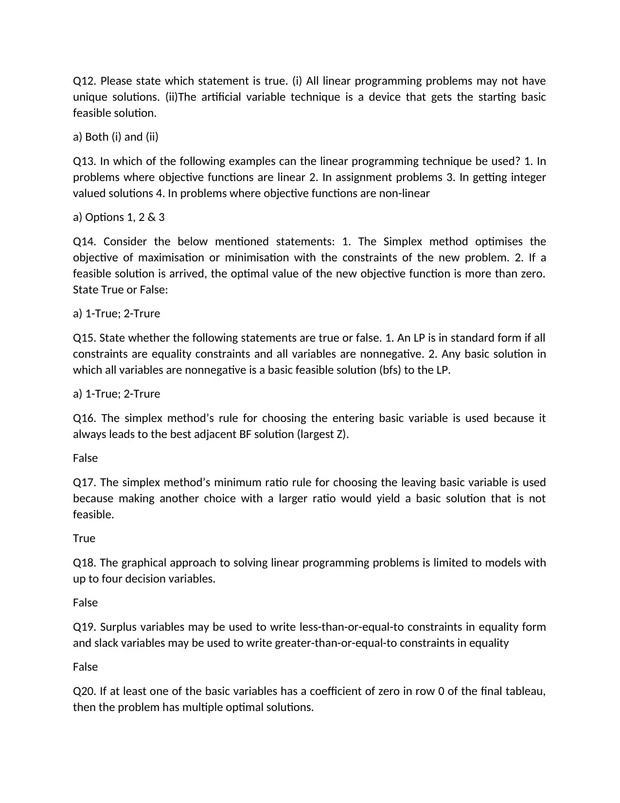
Q12. Please state which statement is true. (i) All linear programming problems may not have
unique solutions. (ii)The artificial variable technique is a device that gets the starting basic
feasible solution.
a) Both (i) and (ii)
Q13. In which of the following examples can the linear programming technique be used? 1. In
problems where objective functions are linear 2. In assignment problems 3. In getting integer
valued solutions 4. In problems where objective functions are non-linear
a) Options 1, 2 & 3
Q14. Consider the below mentioned statements: 1. The Simplex method optimises the
objective of maximisation or minimisation with the constraints of the new problem. 2. If a
feasible solution is arrived, the optimal value of the new objective function is more than zero.
State True or False:
a) 1-True; 2-Trure
Q15. State whether the following statements are true or false. 1. An LP is in standard form if all
constraints are equality constraints and all variables are nonnegative. 2. Any basic solution in
which all variables are nonnegative is a basic feasible solution (bfs) to the LP.
a) 1-True; 2-Trure
Q16. The simplex method’s rule for choosing the entering basic variable is used because it
always leads to the best adjacent BF solution (largest Z).
False
Q17. The simplex method’s minimum ratio rule for choosing the leaving basic variable is used
because making another choice with a larger ratio would yield a basic solution that is not
feasible.
True
Q18. The graphical approach to solving linear programming problems is limited to models with
up to four decision variables.
False
Q19. Surplus variables may be used to write less-than-or-equal-to constraints in equality form
and slack variables may be used to write greater-than-or-equal-to constraints in equality
False
Q20. If at least one of the basic variables has a coefficient of zero in row 0 of the final tableau,
then the problem has multiple optimal solutions.
False
Q21. If the problem has multiple optimal solutions, then the problem must have a bounded
feasible region.
True
Q22. When a linear programming model has an equality constraint, an artificial variable is
introduced into this constraint in order to start the simplex method with an obvious initial basic
solution that is feasible for the original model.
True
Q23. The reduced cost of a variable is equal to the dual value on the non-negativity constraint
for that variable
True
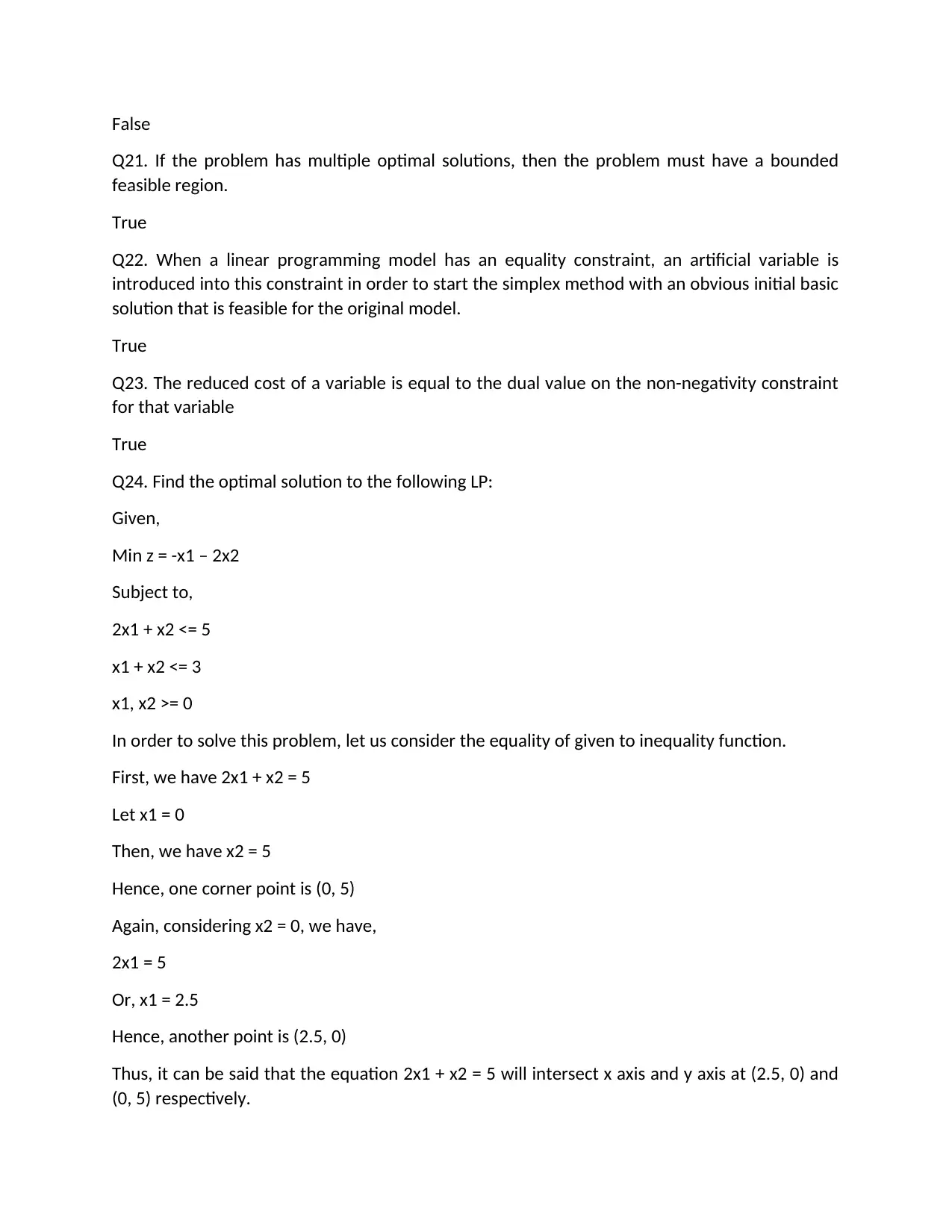
Q24. Find the optimal solution to the following LP:
Given,
Min z = -x1 – 2x2
Subject to,
2x1 + x2 <= 5
x1 + x2 <= 3
x1, x2 >= 0
In order to solve this problem, let us consider the equality of given to inequality function.
First, we have 2x1 + x2 = 5
Let x1 = 0
Then, we have x2 = 5
Hence, one corner point is (0, 5)
Again, considering x2 = 0, we have,
2x1 = 5
Or, x1 = 2.5
Hence, another point is (2.5, 0)
Thus, it can be said that the equation 2x1 + x2 = 5 will intersect x axis and y axis at (2.5, 0) and
(0, 5) respectively.
Secure Best Marks with AI Grader
Need help grading? Try our AI Grader for instant feedback on your assignments.
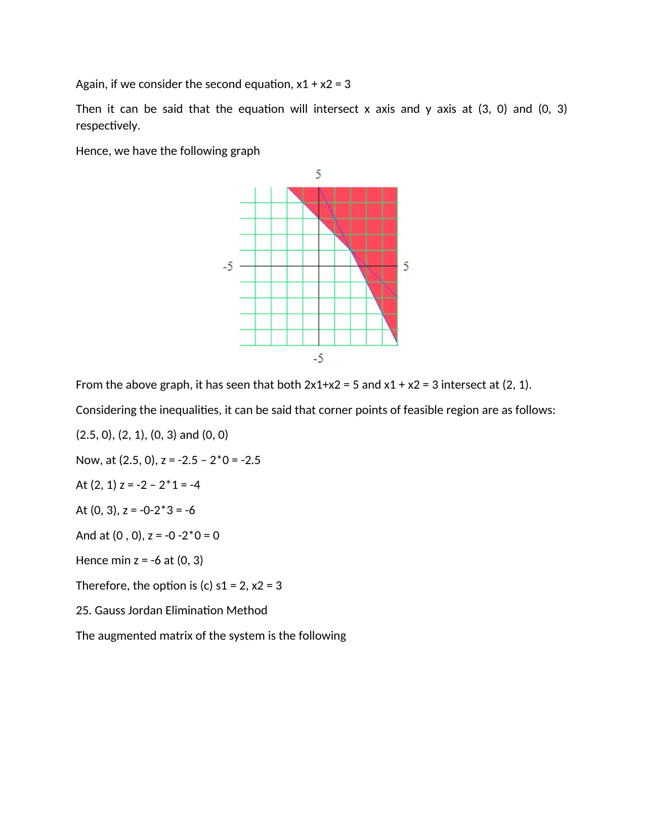
Again, if we consider the second equation, x1 + x2 = 3
Then it can be said that the equation will intersect x axis and y axis at (3, 0) and (0, 3)
respectively.
Hence, we have the following graph
From the above graph, it has seen that both 2x1+x2 = 5 and x1 + x2 = 3 intersect at (2, 1).
Considering the inequalities, it can be said that corner points of feasible region are as follows:
(2.5, 0), (2, 1), (0, 3) and (0, 0)
Now, at (2.5, 0), z = -2.5 – 2*0 = -2.5
At (2, 1) z = -2 – 2*1 = -4
At (0, 3), z = -0-2*3 = -6
And at (0 , 0), z = -0 -2*0 = 0
Hence min z = -6 at (0, 3)
Therefore, the option is (c) s1 = 2, x2 = 3
25. Gauss Jordan Elimination Method
The augmented matrix of the system is the following
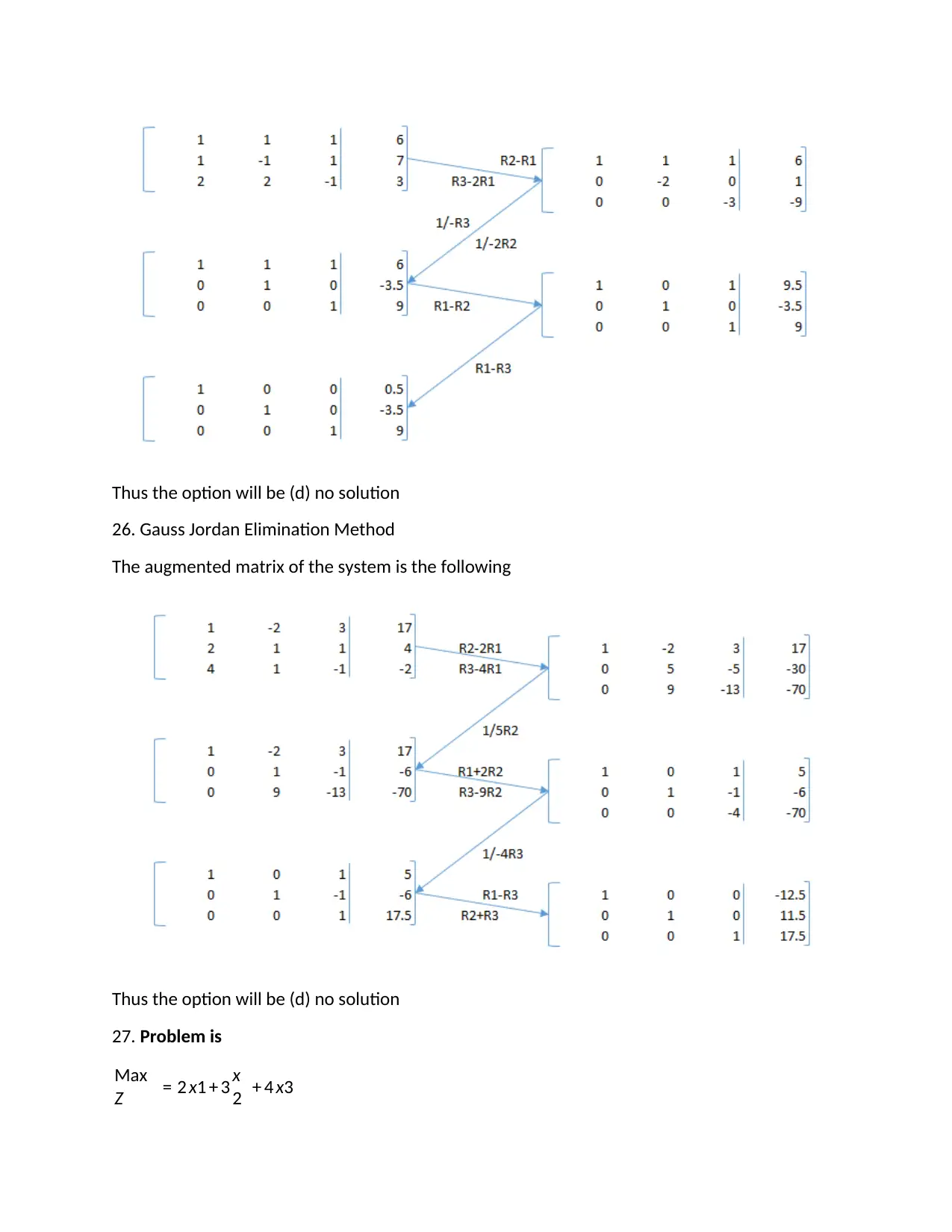
Thus the option will be (d) no solution
26. Gauss Jordan Elimination Method
The augmented matrix of the system is the following
Thus the option will be (d) no solution
27. Problem is
Max
Z = 2 x1 + 3 x
2 + 4 x3
26. Gauss Jordan Elimination Method
The augmented matrix of the system is the following
Thus the option will be (d) no solution
27. Problem is
Max
Z = 2 x1 + 3 x
2 + 4 x3
subject to
3 x1 + 2 x2 - 3 x3 ≤ 4
2 x1 + 3 x2 + 2 x3 ≤ 6
3 x1 - x2 + 2 x3 ≥ -8
Here b3 = -8 < 0,
so multiply this constraint by -1 to make b3 > 0.
- 3 x1 + x2 - 2 x3 ≤ 8
and x1,x2,x3≥0;
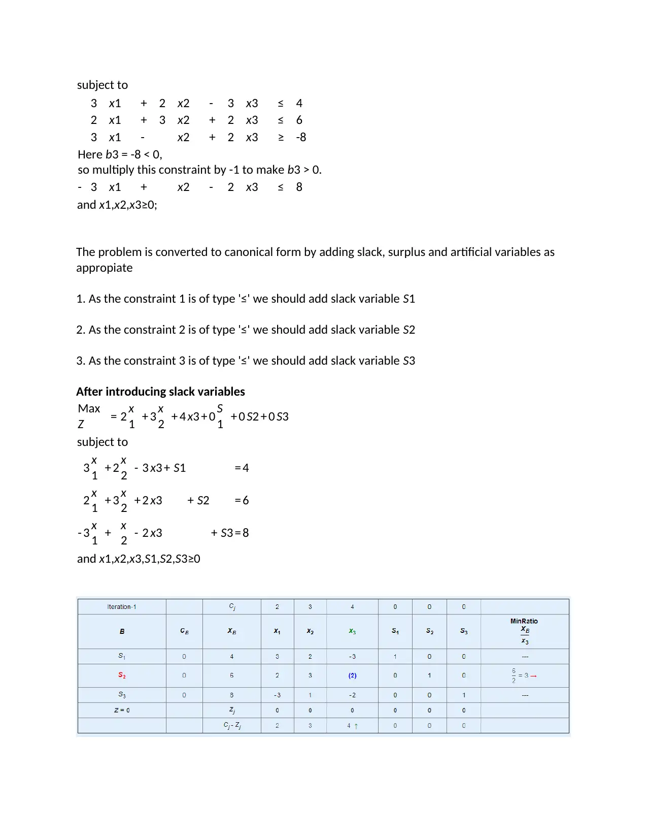
The problem is converted to canonical form by adding slack, surplus and artificial variables as
appropiate
1. As the constraint 1 is of type '≤' we should add slack variable S1
2. As the constraint 2 is of type '≤' we should add slack variable S2
3. As the constraint 3 is of type '≤' we should add slack variable S3
After introducing slack variables
Max
Z = 2 x
1 + 3 x
2 + 4 x3 + 0 S
1 + 0 S2 + 0 S3
subject to
3 x
1 + 2 x
2 - 3 x3 + S1 = 4
2 x
1 + 3 x
2 + 2 x3 + S2 = 6
- 3 x
1 + x
2 - 2 x3 + S3 = 8
and x1,x2,x3,S1,S2,S3≥0
Paraphrase This Document
Need a fresh take? Get an instant paraphrase of this document with our AI Paraphraser
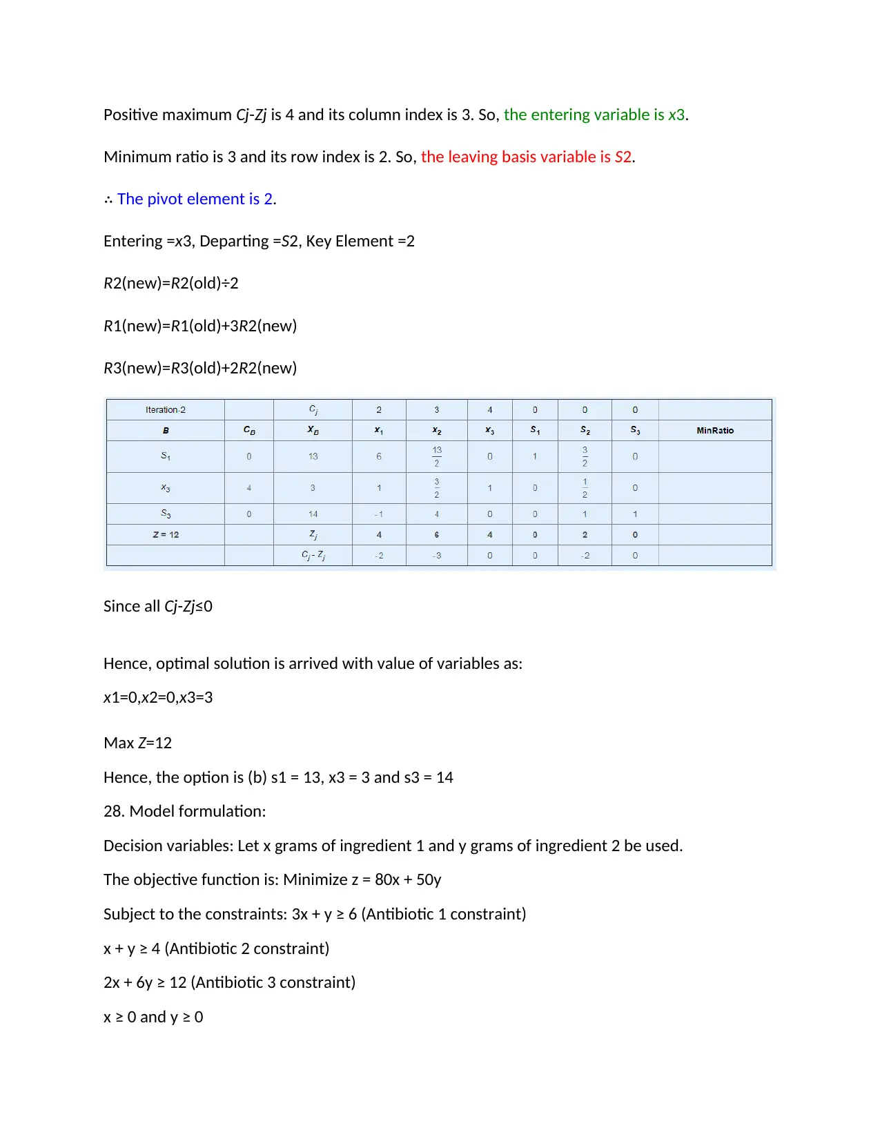
Positive maximum Cj-Zj is 4 and its column index is 3. So, the entering variable is x3.
Minimum ratio is 3 and its row index is 2. So, the leaving basis variable is S2.
∴ The pivot element is 2.
Entering =x3, Departing =S2, Key Element =2
R2(new)=R2(old)÷2
R1(new)=R1(old)+3R2(new)
R3(new)=R3(old)+2R2(new)
Since all Cj-Zj≤0
Hence, optimal solution is arrived with value of variables as:
x1=0,x2=0,x3=3
Max Z=12
Hence, the option is (b) s1 = 13, x3 = 3 and s3 = 14
28. Model formulation:
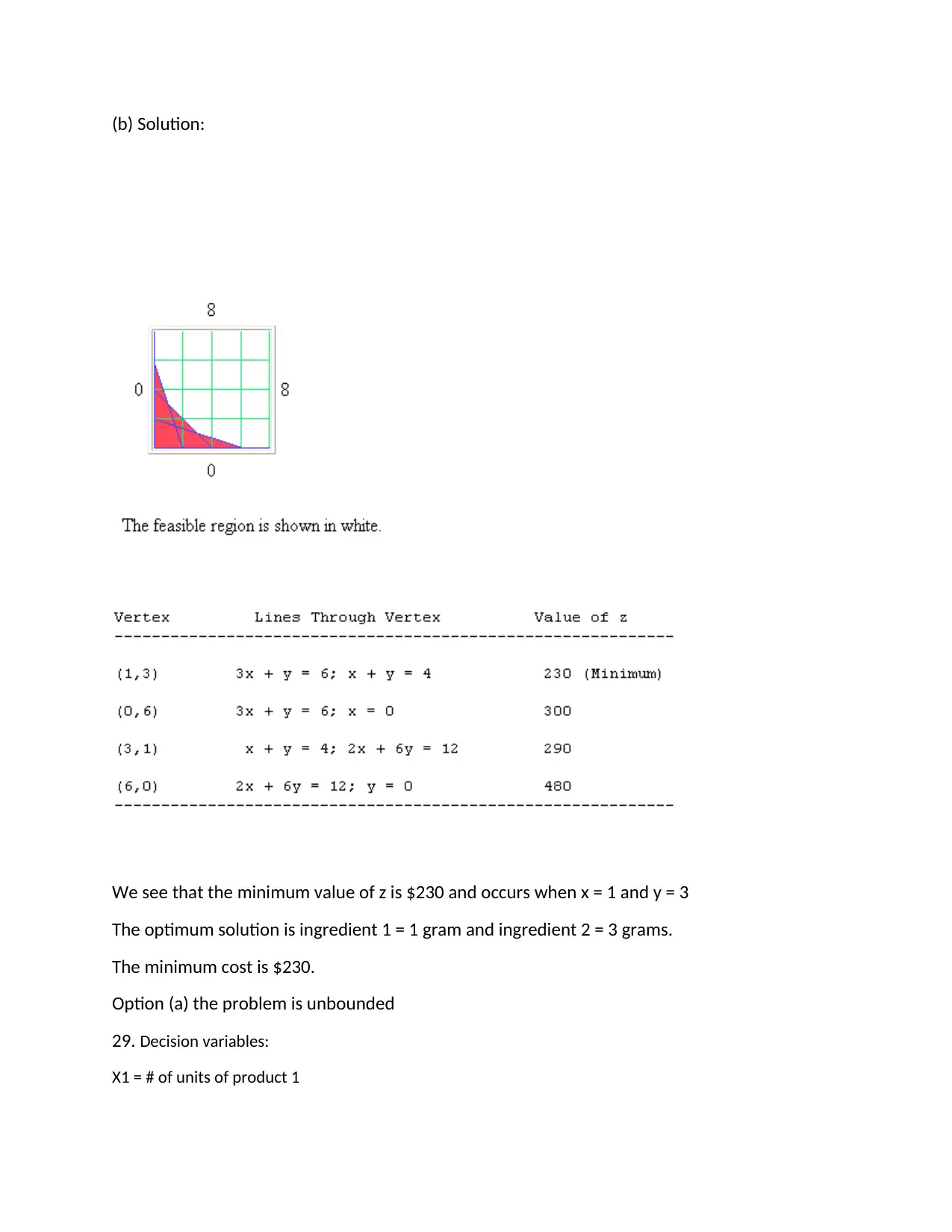
Decision variables: Let x grams of ingredient 1 and y grams of ingredient 2 be used.
The objective function is: Minimize z = 80x + 50y
Subject to the constraints: 3x + y ≥ 6 (Antibiotic 1 constraint)
x + y ≥ 4 (Antibiotic 2 constraint)
2x + 6y ≥ 12 (Antibiotic 3 constraint)
x ≥ 0 and y ≥ 0
(b) Solution:
We see that the minimum value of z is $230 and occurs when x = 1 and y = 3
The optimum solution is ingredient 1 = 1 gram and ingredient 2 = 3 grams.
The minimum cost is $230.
Option (a) the problem is unbounded
29. Decision variables:
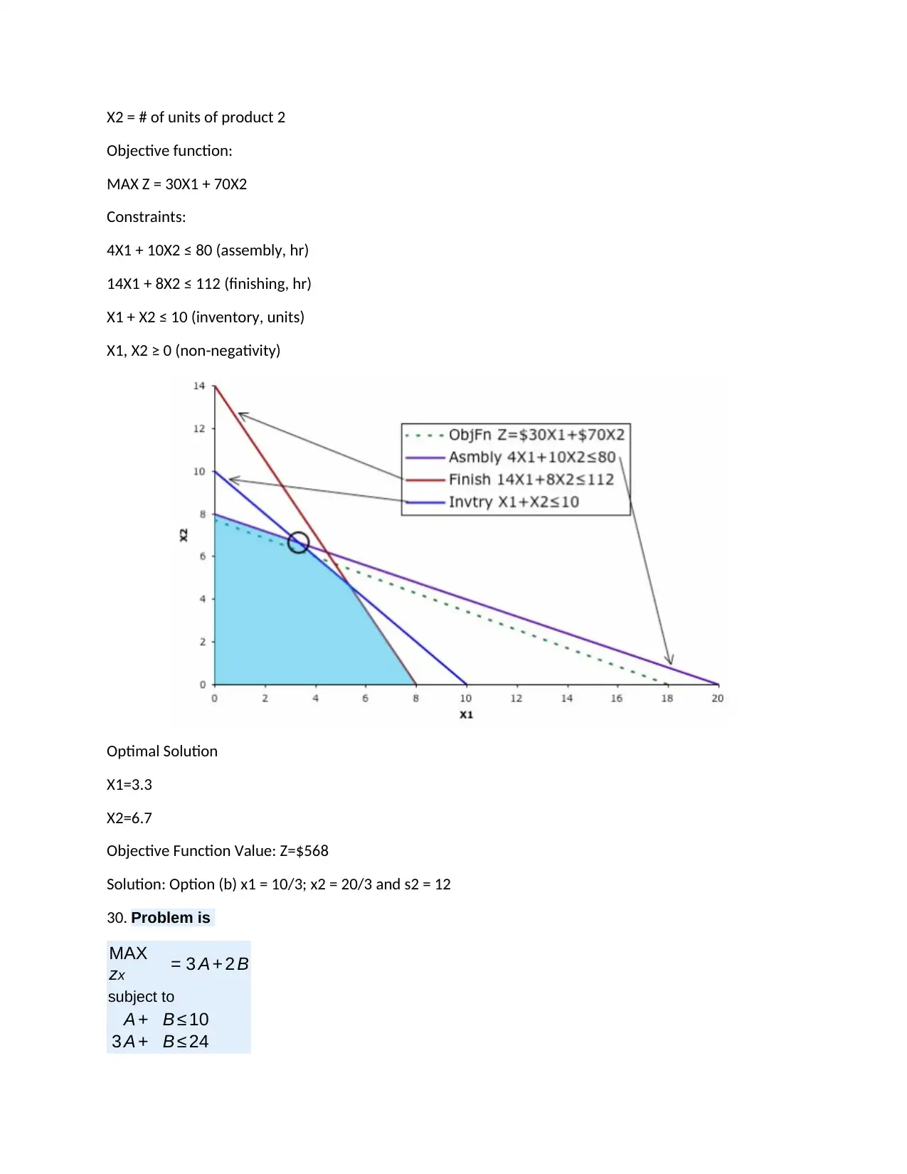
X1 = # of units of product 1
We see that the minimum value of z is $230 and occurs when x = 1 and y = 3
The optimum solution is ingredient 1 = 1 gram and ingredient 2 = 3 grams.
The minimum cost is $230.
Option (a) the problem is unbounded
29. Decision variables:
X1 = # of units of product 1
X2 = # of units of product 2
Objective function:
MAX Z = 30X1 + 70X2
Constraints:
4X1 + 10X2 ≤ 80 (assembly, hr)
14X1 + 8X2 ≤ 112 (finishing, hr)
X1 + X2 ≤ 10 (inventory, units)
X1, X2 ≥ 0 (non-negativity)
Optimal Solution
X1=3.3
X2=6.7
Objective Function Value: Z=$568
Solution: Option (b) x1 = 10/3; x2 = 20/3 and s2 = 12
30. Problem is
MAX
zx = 3 A + 2 B
subject to
A + B ≤ 10
3 A + B ≤ 24
Secure Best Marks with AI Grader
Need help grading? Try our AI Grader for instant feedback on your assignments.
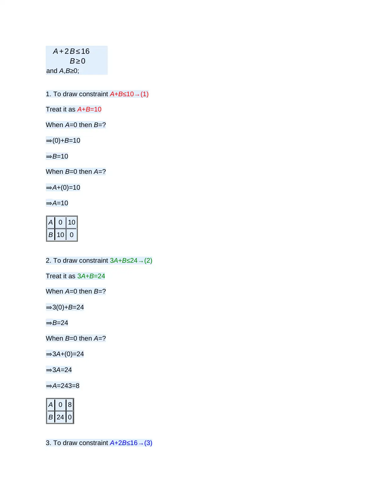
A + 2 B ≤ 16
B ≥ 0
and A,B≥0;
1. To draw constraint A+B≤10→(1)
Treat it as A+B=10
When A=0 then B=?
⇒(0)+B=10
⇒B=10
When B=0 then A=?
⇒A+(0)=10
⇒A=10
A 0 10
B 10 0
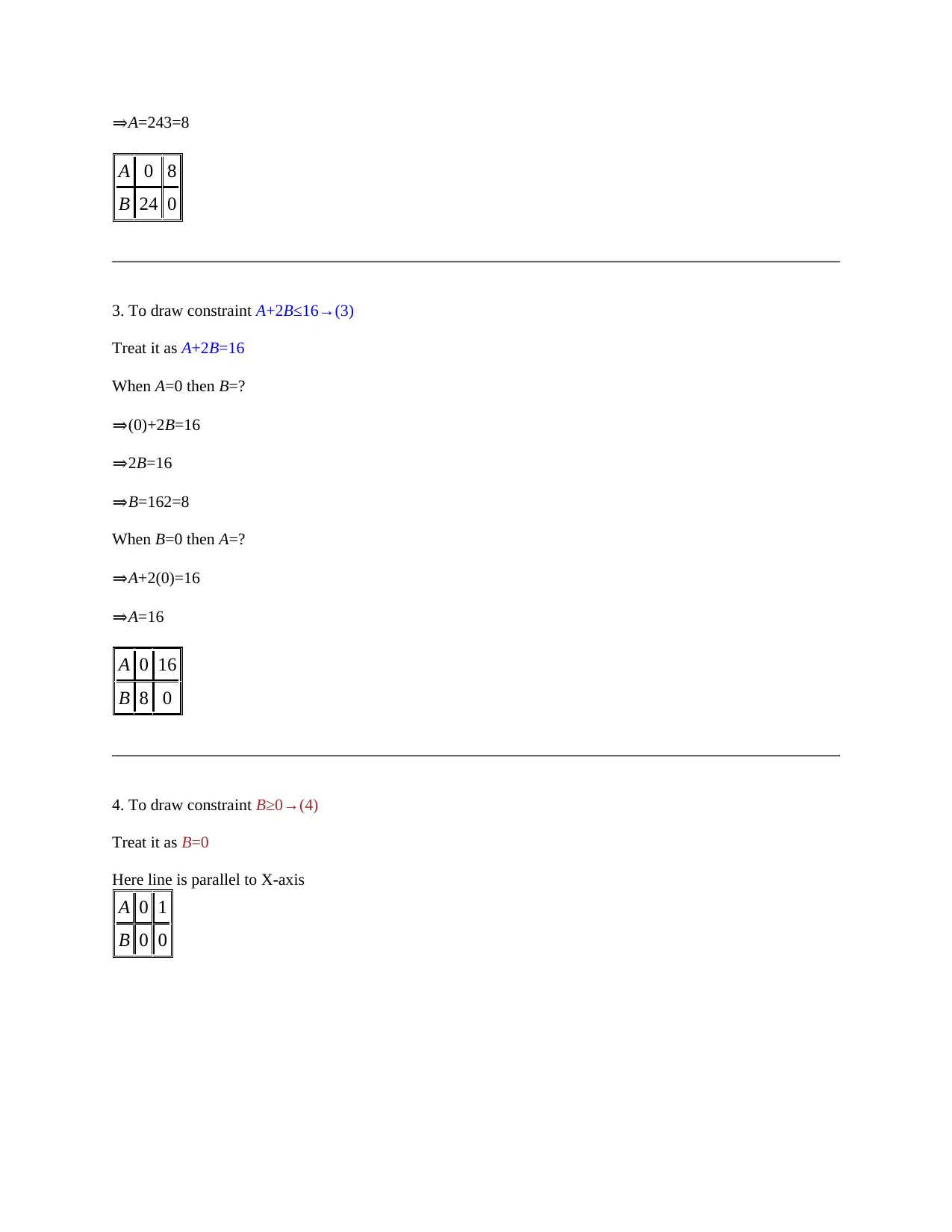
2. To draw constraint 3A+B≤24→(2)
Treat it as 3A+B=24
When A=0 then B=?
⇒3(0)+B=24
⇒B=24
When B=0 then A=?
⇒3A+(0)=24
⇒3A=24
⇒A=243=8
A 0 8
B 24 0
3. To draw constraint A+2B≤16→(3)
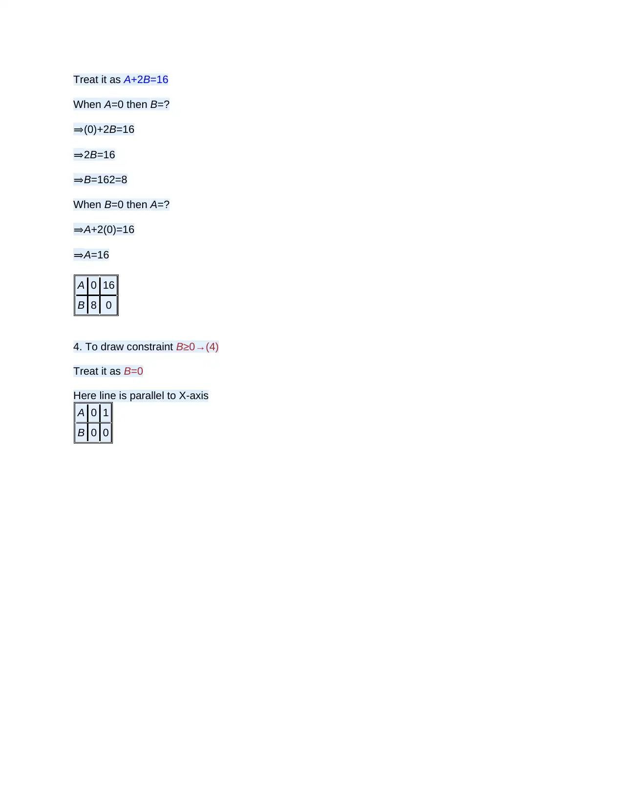
Treat it as A+2B=16
When A=0 then B=?
⇒(0)+2B=16
⇒2B=16
⇒B=162=8
When B=0 then A=?
⇒A+2(0)=16
⇒A=16
A 0 16
B 8 0
4. To draw constraint B≥0→(4)
Treat it as B=0
Here line is parallel to X-axis
A 0 1
B 0 0
When A=0 then B=?
⇒(0)+2B=16
⇒2B=16
⇒B=162=8
When B=0 then A=?
⇒A+2(0)=16
⇒A=16
A 0 16
B 8 0
4. To draw constraint B≥0→(4)
Treat it as B=0
Here line is parallel to X-axis
A 0 1
B 0 0
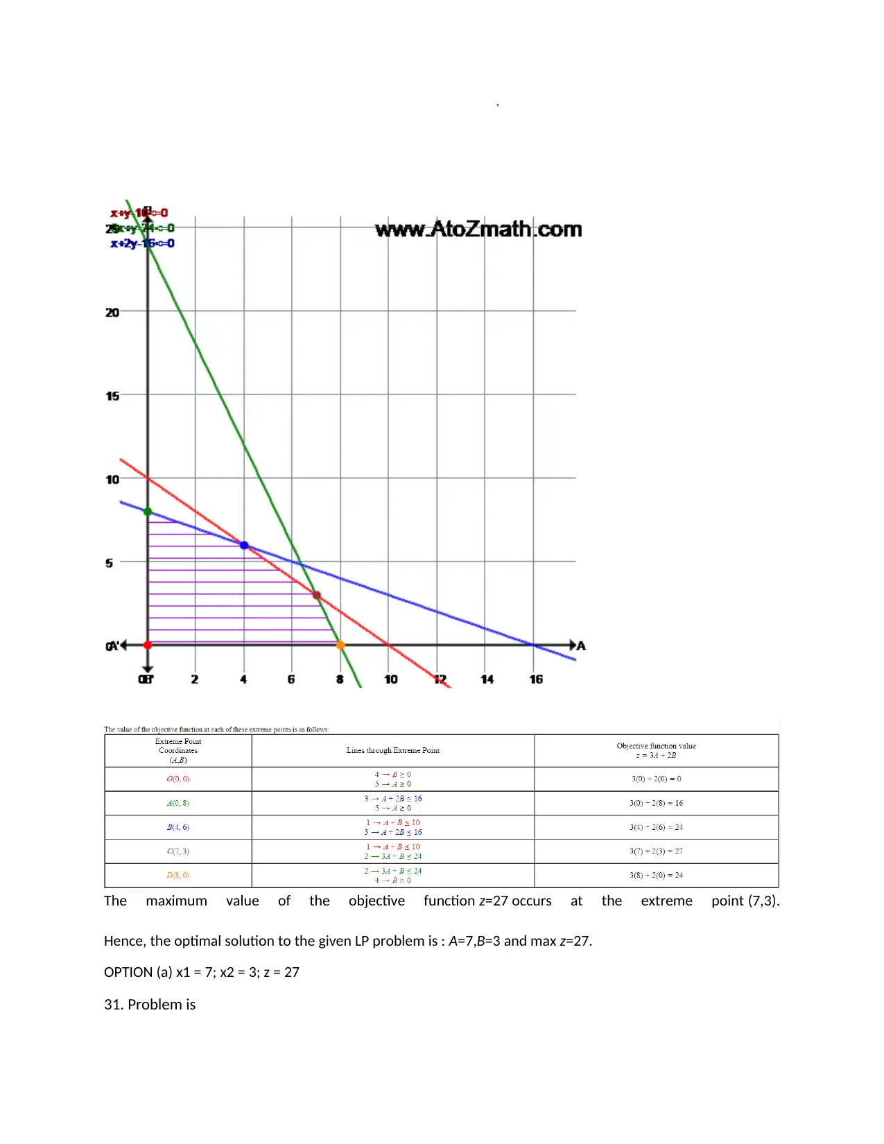
The maximum value of the objective function z=27 occurs at the extreme point (7,3).
Hence, the optimal solution to the given LP problem is : A=7,B=3 and max z=27.
OPTION (a) x1 = 7; x2 = 3; z = 27
31. Problem is
Hence, the optimal solution to the given LP problem is : A=7,B=3 and max z=27.
OPTION (a) x1 = 7; x2 = 3; z = 27
31. Problem is
Paraphrase This Document
Need a fresh take? Get an instant paraphrase of this document with our AI Paraphraser
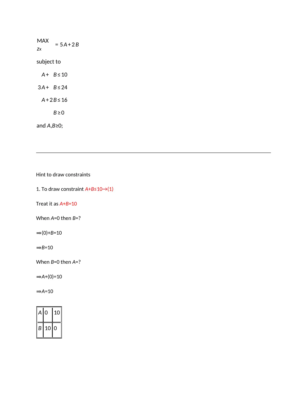
MAX
zx = 5 A + 2 B
subject to
A + B ≤ 10
3 A + B ≤ 24
A + 2 B ≤ 16
B ≥ 0
and A,B≥0;
Hint to draw constraints
1. To draw constraint A+B≤10→(1)
Treat it as A+B=10
When A=0 then B=?
⇒(0)+B=10
⇒B=10
When B=0 then A=?
⇒A+(0)=10
⇒A=10
A 0 10
B 10 0
zx = 5 A + 2 B
subject to
A + B ≤ 10
3 A + B ≤ 24
A + 2 B ≤ 16
B ≥ 0
and A,B≥0;
Hint to draw constraints
1. To draw constraint A+B≤10→(1)
Treat it as A+B=10
When A=0 then B=?
⇒(0)+B=10
⇒B=10
When B=0 then A=?
⇒A+(0)=10
⇒A=10
A 0 10
B 10 0
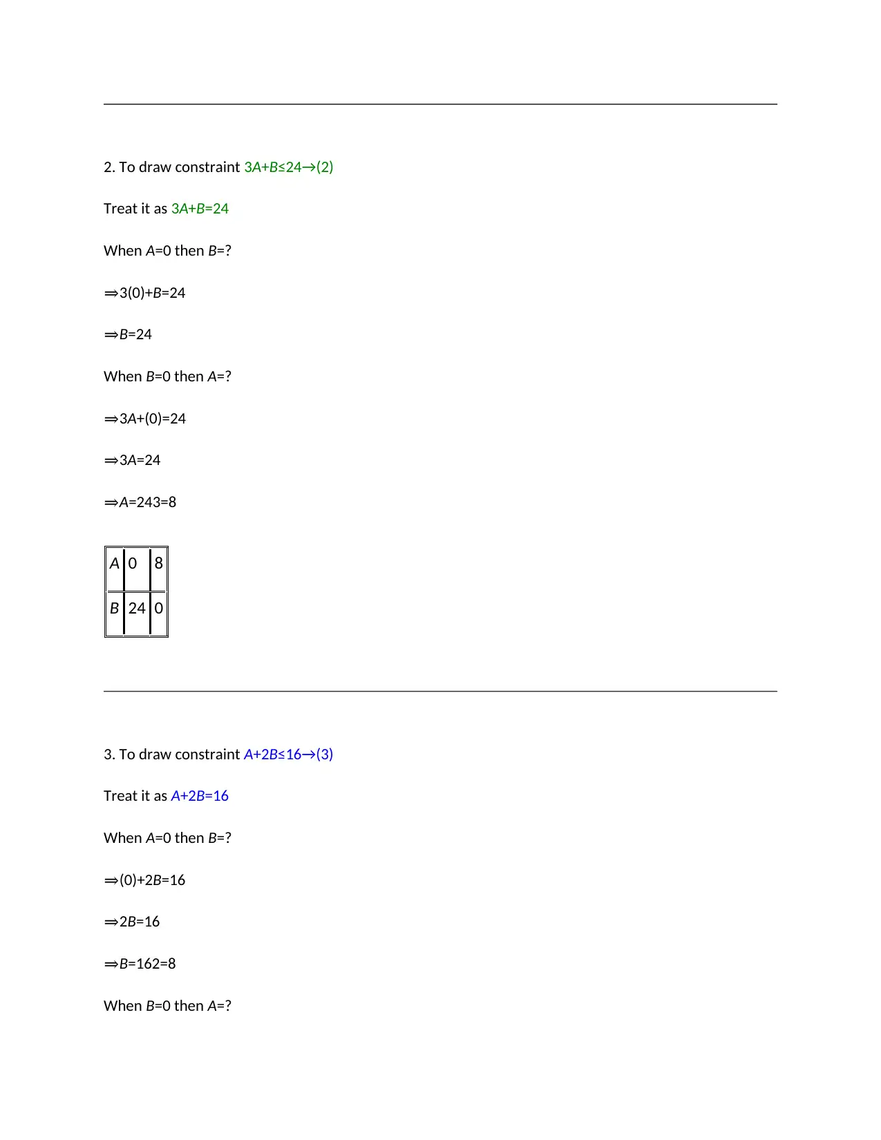
2. To draw constraint 3A+B≤24→(2)
Treat it as 3A+B=24
When A=0 then B=?
⇒3(0)+B=24
⇒B=24
When B=0 then A=?
⇒3A+(0)=24
⇒3A=24
⇒A=243=8
A 0 8
B 24 0
3. To draw constraint A+2B≤16→(3)
Treat it as A+2B=16
When A=0 then B=?
⇒(0)+2B=16
⇒2B=16
⇒B=162=8
When B=0 then A=?
Treat it as 3A+B=24
When A=0 then B=?
⇒3(0)+B=24
⇒B=24
When B=0 then A=?
⇒3A+(0)=24
⇒3A=24
⇒A=243=8
A 0 8
B 24 0
3. To draw constraint A+2B≤16→(3)
Treat it as A+2B=16
When A=0 then B=?
⇒(0)+2B=16
⇒2B=16
⇒B=162=8
When B=0 then A=?
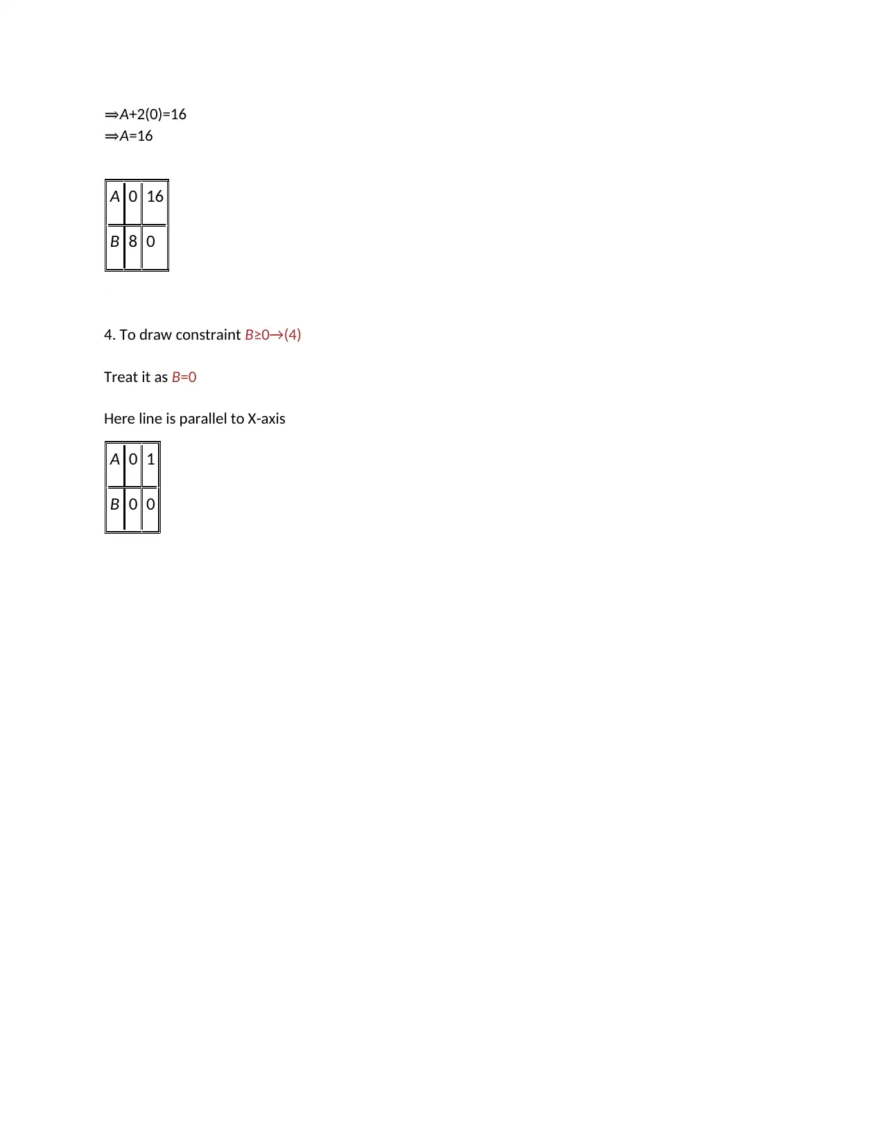
⇒A+2(0)=16
⇒A=16
A 0 16
B 8 0
4. To draw constraint B≥0→(4)
Treat it as B=0
Here line is parallel to X-axis
A 0 1
B 0 0
⇒A=16
A 0 16
B 8 0
4. To draw constraint B≥0→(4)
Treat it as B=0
Here line is parallel to X-axis
A 0 1
B 0 0
Secure Best Marks with AI Grader
Need help grading? Try our AI Grader for instant feedback on your assignments.
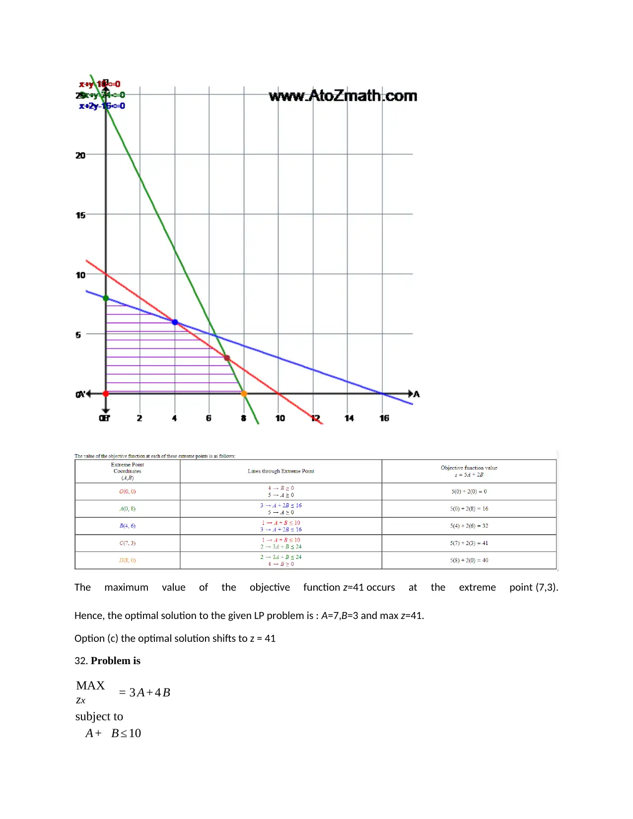
The maximum value of the objective function z=41 occurs at the extreme point (7,3).
Hence, the optimal solution to the given LP problem is : A=7,B=3 and max z=41.
Option (c) the optimal solution shifts to z = 41
32. Problem is
MAX
zx = 3 A + 4 B
subject to
A + B ≤ 10
Hence, the optimal solution to the given LP problem is : A=7,B=3 and max z=41.
Option (c) the optimal solution shifts to z = 41
32. Problem is
MAX
zx = 3 A + 4 B
subject to
A + B ≤ 10
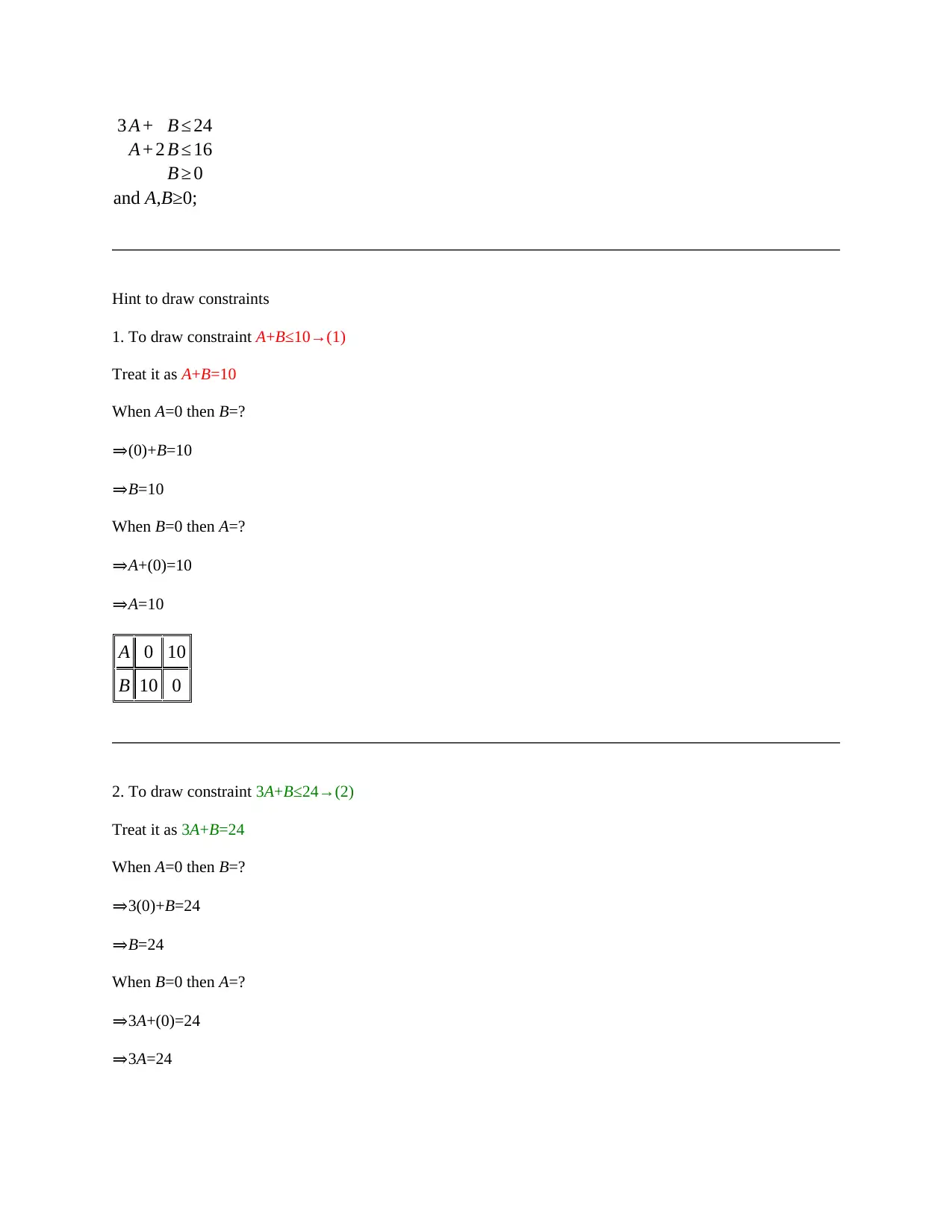
3 A + B ≤ 24
A + 2 B ≤ 16
B ≥ 0
and A,B≥0;
Hint to draw constraints
1. To draw constraint A+B≤10→(1)
Treat it as A+B=10
When A=0 then B=?
⇒(0)+B=10
⇒B=10
When B=0 then A=?
⇒A+(0)=10
⇒A=10
A 0 10
B 10 0
2. To draw constraint 3A+B≤24→(2)
Treat it as 3A+B=24
When A=0 then B=?
⇒3(0)+B=24
⇒B=24
When B=0 then A=?
⇒3A+(0)=24
⇒3A=24

⇒A=243=8
A 0 8
B 24 0
3. To draw constraint A+2B≤16→(3)
Treat it as A+2B=16
When A=0 then B=?
⇒(0)+2B=16
⇒2B=16
⇒B=162=8
When B=0 then A=?
⇒A+2(0)=16
⇒A=16
A 0 16
B 8 0
4. To draw constraint B≥0→(4)
Treat it as B=0
Here line is parallel to X-axis
A 0 1
B 0 0
A 0 8
B 24 0
3. To draw constraint A+2B≤16→(3)
Treat it as A+2B=16
When A=0 then B=?
⇒(0)+2B=16
⇒2B=16
⇒B=162=8
When B=0 then A=?
⇒A+2(0)=16
⇒A=16
A 0 16
B 8 0
4. To draw constraint B≥0→(4)
Treat it as B=0
Here line is parallel to X-axis
A 0 1
B 0 0
Paraphrase This Document
Need a fresh take? Get an instant paraphrase of this document with our AI Paraphraser
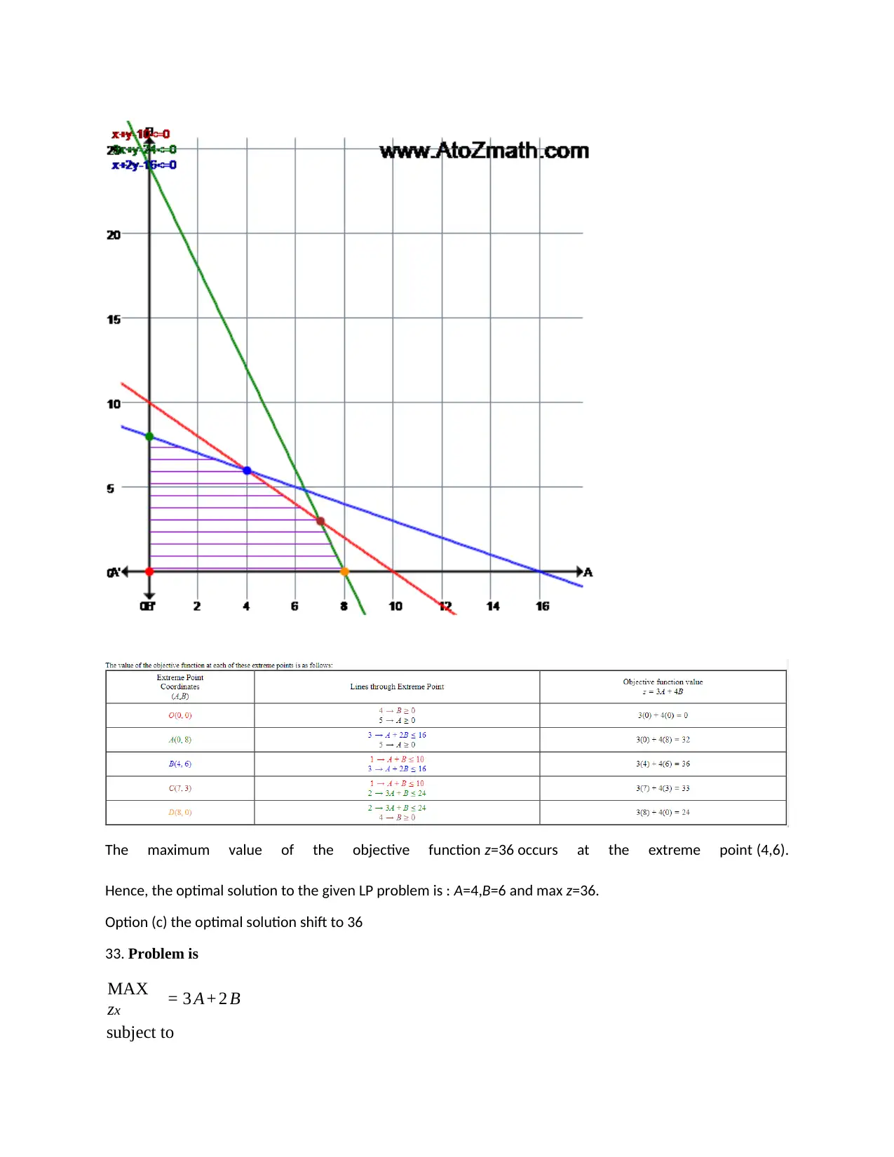
The maximum value of the objective function z=36 occurs at the extreme point (4,6).
Hence, the optimal solution to the given LP problem is : A=4,B=6 and max z=36.
Option (c) the optimal solution shift to 36
33. Problem is
MAX
zx = 3 A + 2 B
subject to
Hence, the optimal solution to the given LP problem is : A=4,B=6 and max z=36.
Option (c) the optimal solution shift to 36
33. Problem is
MAX
zx = 3 A + 2 B
subject to
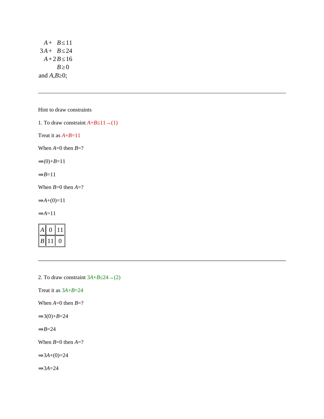
A + B ≤ 11
3 A + B ≤ 24
A + 2 B ≤ 16
B ≥ 0
and A,B≥0;
Hint to draw constraints
1. To draw constraint A+B≤11→(1)
Treat it as A+B=11
When A=0 then B=?
⇒(0)+B=11
⇒B=11
When B=0 then A=?
⇒A+(0)=11
⇒A=11
A 0 11
B 11 0
2. To draw constraint 3A+B≤24→(2)
Treat it as 3A+B=24
When A=0 then B=?
⇒3(0)+B=24
⇒B=24
When B=0 then A=?
⇒3A+(0)=24
⇒3A=24
⇒A=243=8
A 0 8
B 24 0
3. To draw constraint A+2B≤16→(3)
Treat it as A+2B=16
When A=0 then B=?
⇒(0)+2B=16
⇒2B=16
⇒B=162=8
When B=0 then A=?
⇒A+2(0)=16
⇒A=16
A 0 16
B 8 0
4. To draw constraint B≥0→(4)
Treat it as B=0
Here line is parallel to X-axis
A 0 1
B 0 0
A 0 8
B 24 0
3. To draw constraint A+2B≤16→(3)
Treat it as A+2B=16
When A=0 then B=?
⇒(0)+2B=16
⇒2B=16
⇒B=162=8
When B=0 then A=?
⇒A+2(0)=16
⇒A=16
A 0 16
B 8 0
4. To draw constraint B≥0→(4)
Treat it as B=0
Here line is parallel to X-axis
A 0 1
B 0 0
Secure Best Marks with AI Grader
Need help grading? Try our AI Grader for instant feedback on your assignments.
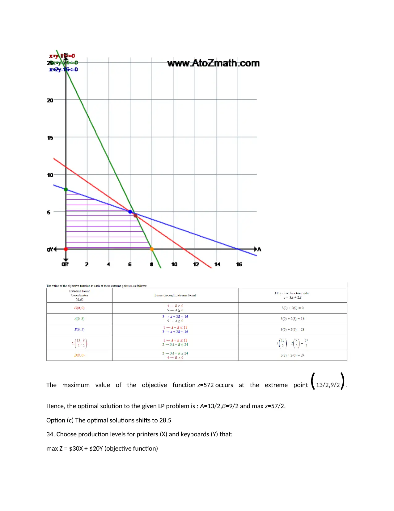
The maximum value of the objective function z=572 occurs at the extreme point (13/2,9/2).
Hence, the optimal solution to the given LP problem is : A=13/2,B=9/2 and max z=57/2.
Option (c) The optimal solutions shifts to 28.5
34. Choose production levels for printers (X) and keyboards (Y) that:
max Z = $30X + $20Y (objective function)
Hence, the optimal solution to the given LP problem is : A=13/2,B=9/2 and max z=57/2.
Option (c) The optimal solutions shifts to 28.5
34. Choose production levels for printers (X) and keyboards (Y) that:
max Z = $30X + $20Y (objective function)
and satisfy the following:
2X + Y <= 1,000 (soldering time constraint)
X + Y <= 800 (assembling time constraint)
X <= 350 (demand constraint for printers)
X => 0 (sign restriction)
Y => 0 (sign restriction)
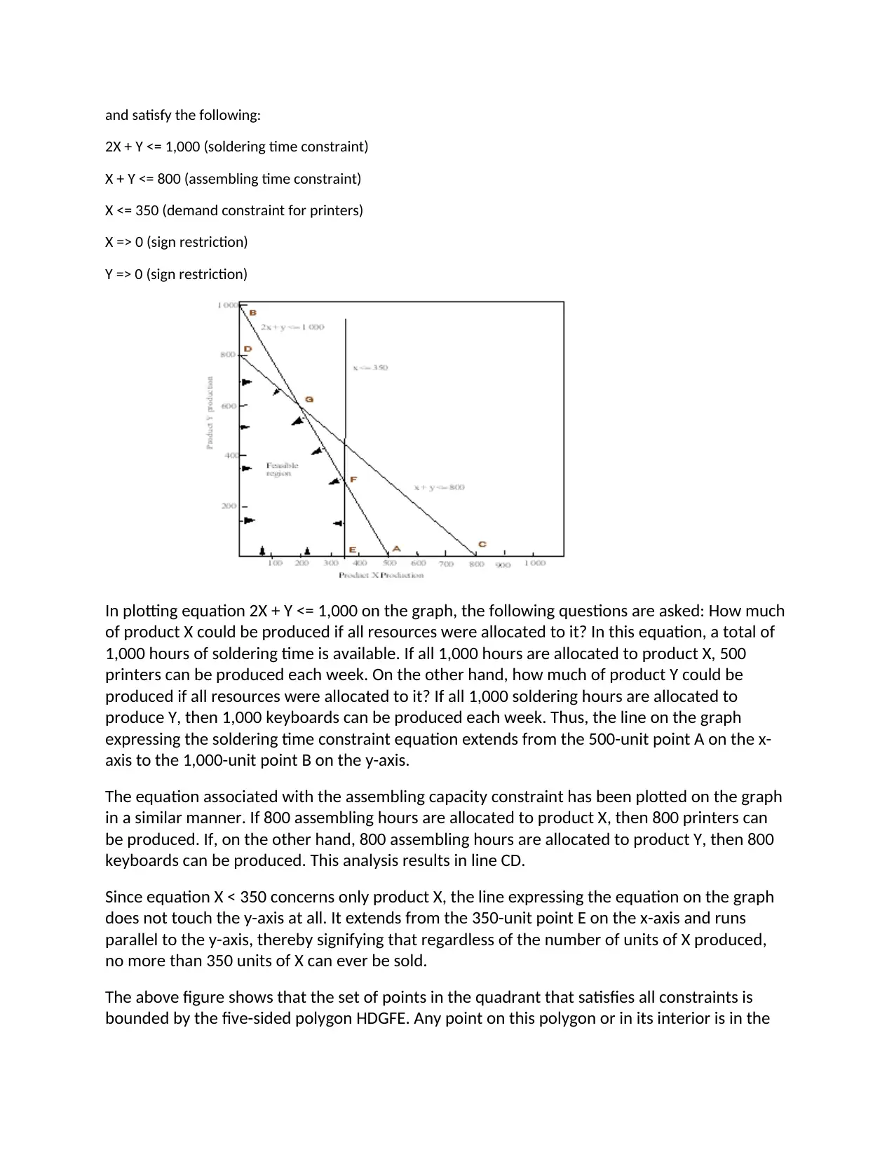
In plotting equation 2X + Y <= 1,000 on the graph, the following questions are asked: How much
of product X could be produced if all resources were allocated to it? In this equation, a total of
1,000 hours of soldering time is available. If all 1,000 hours are allocated to product X, 500
printers can be produced each week. On the other hand, how much of product Y could be
produced if all resources were allocated to it? If all 1,000 soldering hours are allocated to
produce Y, then 1,000 keyboards can be produced each week. Thus, the line on the graph
expressing the soldering time constraint equation extends from the 500-unit point A on the x-
axis to the 1,000-unit point B on the y-axis.
The equation associated with the assembling capacity constraint has been plotted on the graph
in a similar manner. If 800 assembling hours are allocated to product X, then 800 printers can
be produced. If, on the other hand, 800 assembling hours are allocated to product Y, then 800
keyboards can be produced. This analysis results in line CD.
Since equation X < 350 concerns only product X, the line expressing the equation on the graph
does not touch the y-axis at all. It extends from the 350-unit point E on the x-axis and runs
parallel to the y-axis, thereby signifying that regardless of the number of units of X produced,
no more than 350 units of X can ever be sold.
The above figure shows that the set of points in the quadrant that satisfies all constraints is
bounded by the five-sided polygon HDGFE. Any point on this polygon or in its interior is in the
feasible region. Any other point fails to satisfy at least one of the inequalities and thus falls
outside the feasible region.
Having identified the feasible region for the Bridgeway case, we now search for the optimal
solution, which will be the point in the feasible region that maximizes the objective function. In
Bridgeway's case, this is:
max Z = $30X + $20Y
To find the optimal solution, we graph lines so that all points on a particular line have the same
Z-value. In a maximization problem, such lines are called isoprofit lines; in a minimization
problem, they are called isocost lines. The parallel lines are created by assigning various values
to Z in the objective function to provide either higher profits or lower costs.
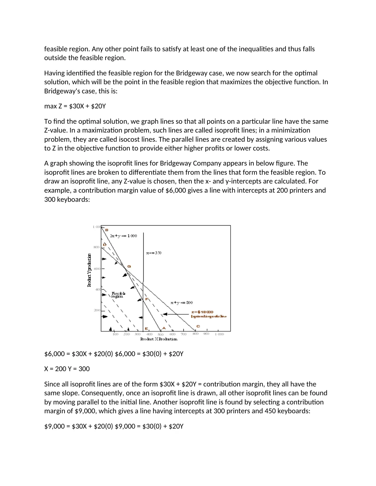
A graph showing the isoprofit lines for Bridgeway Company appears in below figure. The
isoprofit lines are broken to differentiate them from the lines that form the feasible region. To
draw an isoprofit line, any Z-value is chosen, then the x- and y-intercepts are calculated. For
example, a contribution margin value of $6,000 gives a line with intercepts at 200 printers and
300 keyboards:
$6,000 = $30X + $20(0) $6,000 = $30(0) + $20Y
X = 200 Y = 300
Since all isoprofit lines are of the form $30X + $20Y = contribution margin, they all have the
same slope. Consequently, once an isoprofit line is drawn, all other isoprofit lines can be found
by moving parallel to the initial line. Another isoprofit line is found by selecting a contribution
margin of $9,000, which gives a line having intercepts at 300 printers and 450 keyboards:
$9,000 = $30X + $20(0) $9,000 = $30(0) + $20Y
Paraphrase This Document
Need a fresh take? Get an instant paraphrase of this document with our AI Paraphraser
X = 300 Y = 450
Isoprofit lines move in a northeast direction; that is, upward and to the right. After a while, the
isoprofit lines will no longer intersect the feasible region. The isoprofit line intersecting the last
vertex of the feasible region defines the largest Z-value of any point in the feasible region and
indicates the optimal solution to the LP problem. In Exhibit 16-3, the isoprofit line passing
through point G is the last isoprofit line to intersect the feasible region. Thus, point G is the
point in the feasible region with the largest Z-value and is therefore the optimal solution to the
Bridgeway problem. Note that point G is located at the intersection of lines 2X + Y = 1,000 and X
+ Y = 800. Solving these two equations simultaneously results in:
X = 200
Y = 600
The optimal value of Z (i.e., the total contribution margin) may be found by substituting these
values of X and Y into the objective function. Thus, the optimal value of Z is:
max Z = $30 (200) + $20 (600) = $18,000
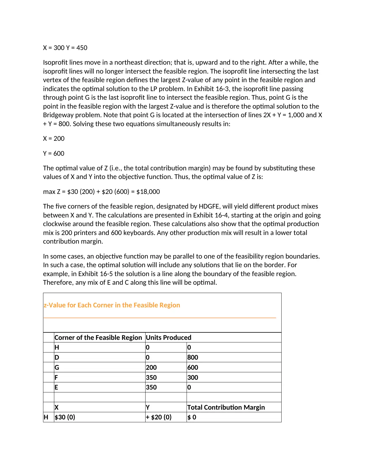
The five corners of the feasible region, designated by HDGFE, will yield different product mixes
between X and Y. The calculations are presented in Exhibit 16-4, starting at the origin and going
clockwise around the feasible region. These calculations also show that the optimal production
mix is 200 printers and 600 keyboards. Any other production mix will result in a lower total
contribution margin.
In some cases, an objective function may be parallel to one of the feasibility region boundaries.
In such a case, the optimal solution will include any solutions that lie on the border. For
example, in Exhibit 16-5 the solution is a line along the boundary of the feasible region.
Therefore, any mix of E and C along this line will be optimal.
z-Value for Each Corner in the Feasible Region
Corner of the Feasible Region Units Produced
H 0 0
D 0 800
G 200 600
F 350 300
E 350 0
X Y Total Contribution Margin
H $30 (0) + $20 (0) $ 0
1 out of 26
Related Documents
Your All-in-One AI-Powered Toolkit for Academic Success.
+13062052269
info@desklib.com
Available 24*7 on WhatsApp / Email
![[object Object]](/_next/static/media/star-bottom.7253800d.svg)
Unlock your academic potential
© 2024 | Zucol Services PVT LTD | All rights reserved.


