BFM102B - Valuation of Investments 1: Comprehensive Assignment
VerifiedAdded on 2022/12/22
|11
|3031
|2
Homework Assignment
AI Summary
This document presents a comprehensive solution to a BFM102B Valuation of Investments assignment. It begins by explaining the marking-to-market process for futures contracts and then proceeds to calculate forward prices, considering dividend yields and risk-free rates. The solution also explores various options strategies, including stop-loss orders, hedging techniques, and the valuation of call options. Furthermore, it delves into the concepts of knock-in options, barrier options, and their valuation. The assignment includes calculations for portfolio deltas, gammas, and vegas, and concludes with an analysis of bull and bear spreads using call and put options. Finally, it discusses the assumptions underlying the Black-Scholes model and their impact on option pricing, providing a thorough understanding of investment valuation principles.
BFM102B - Valuation of Investments
1
1
Paraphrase This Document
Need a fresh take? Get an instant paraphrase of this document with our AI Paraphraser
Contents
BFM102B - Valuation of Investments.............................................................................................1
Contents...........................................................................................................................................2
QUESTION 1...................................................................................................................................3
(a) Describe the marking-to-market process for futures contracts:.............................................3
(b)................................................................................................................................................3
(c)................................................................................................................................................4
QUESTION 2...................................................................................................................................5
(a)................................................................................................................................................5
(b)................................................................................................................................................6
(c)................................................................................................................................................7
(d)................................................................................................................................................8
Question 3........................................................................................................................................9
References......................................................................................................................................11
2
QUESTION 1
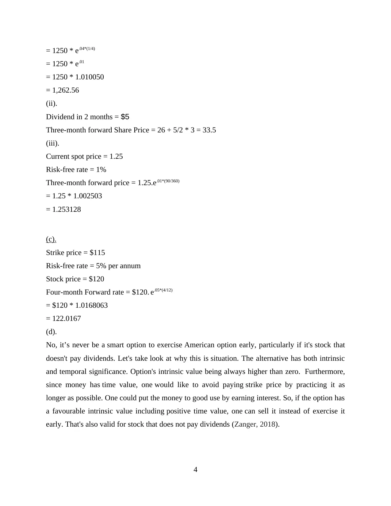
(a) Describe the marking-to-market process for futures contracts:
Gains as well as losses settled on every trading day, which is one of most significant aspects of
futures contracts/transactions. Mark to Market settlement is the term for this method. This
implies that contract's value has been adjusted to reflect its actual market value. The
exchanges will receive this MTM margins from loss-bearing party as well as pay this to gain-
eligible recipient party with support of brokers or clearing houses (Raimbourg and Zimmermann,
2018).
MTM stands for mark to market, as well as this is a way of determining fair value of
accounts which vary over period, like assets and liabilities. The objective of marks to market
would provide a practical assessment of a business's or organization's current financial position
based on existing market conditions. Depending on what the business could expect in return
for asset under present industry conditions marks to market will provide a more reliable figure
for current value of company's assets.
MTM cannot accurately reflect asset's true value in orderly market throughout adverse or
unpredictable times. Marks to market is in comparison to historical costs accounting that
keeps asset's value at its purchasing price. Transactions for futures contract being marked to
market on regular in futures trading. Between long and short-positions, profits and losses are
measured (Thirumagal and SURESH, 2019).
Marks to market is accounting concept that refers to the process of changing the valuation
of asset to represent its existing market value. MV of an asset is measured by the amount a
business would receive if it were sold at a certain period. A corporation 's balance sheet should
represent current market value of such accounts at end of fiscal period. Other accounts can keep
their historical expense, which is asset's initial purchasing price.
(b).
(i).
Risk-free rate = 2% p.a.
Dividend yield = 6% per annum
3 Month forward price = F0 = S0 e(r–q )T
= 1250 * e.04*(3/12)
3
⊘ This is a preview!⊘
Do you want full access?
Subscribe today to unlock all pages.
Trusted by 1+ million students worldwide
= 1250 * e.04*(1/4)
= 1250 * e.01
= 1250 * 1.010050
= 1,262.56
(ii).
Dividend in 2 months = $5
Three-month forward Share Price = 26 + 5/2 * 3 = 33.5
(iii).
Current spot price = 1.25
Risk-free rate = 1%
Three-month forward price = 1.25.e.01*(90/360)
= 1.25 * 1.002503
= 1.253128
(c).
Strike price = $115
Risk-free rate = 5% per annum
Stock price = $120
Four-month Forward rate = $120. e.05*(4/12)
= $120 * 1.0168063
= 122.0167
(d).
No, it’s never be a smart option to exercise American option early, particularly if it's stock that
doesn't pay dividends. Let's take look at why this is situation. The alternative has both intrinsic
and temporal significance. Option's intrinsic value being always higher than zero. Furthermore,
since money has time value, one would like to avoid paying strike price by practicing it as
longer as possible. One could put the money to good use by earning interest. So, if the option has
a favourable intrinsic value including positive time value, one can sell it instead of exercise it
early. That's also valid for stock that does not pay dividends (Zanger, 2018).
4
Paraphrase This Document
Need a fresh take? Get an instant paraphrase of this document with our AI Paraphraser
QUESTION 2
(a).
Stop-loss strategy:
Stop-loss strategy being used to determine when an investor can sell stock or security. That's a
stopping order with a listed price that's lower than current market price which is intended to be
selling. Stop-losses are mostly employed to protect traders' longer positions when hedging
(Ciorciari, 2019).
Hedging:
Regulating or reducing risks is what hedging is all about. Hedge is term for investment strategy
that uses another investment to hedge future gains and losses.
Out-of-the-money call options:
If strike price of call option is higher than market price of underlying asset/security, option is
said to be out-of-the-money. That means that investor has the option to buy security at a greater
price than market price, as long as the difference isn't too big. Time value determines price of
out-of-money call options (Haaland, Wright, Tufto and Ratikainen, 2019).
Call options:
Call option offers option holder's right to buy a security at set price if the buyer expects stock
prices would increase.
Suppose the strike price is 10.00. Option writer targets to fully covered if options are in
money as well as naked if this is out-of-money. Option writer tries to accomplish this by
purchasing assets underlying option as early as asset price hits 10.00 from underneath and selling
when asset price crosses 10.00 through above. The problem with this strategy is that this believes
that if asset price increases from 9.99 to then, it can move to higher price. (In reality, it's possible
that the next jump will be 9.99.) It is therefore assumed that if asset price rises from 10.01 to
ten, next move would be under 10.00. Buying at 10.01 as well as selling at the 9.99 is how the
scheme operates. It is, though, a poor hedging. Trading strategy's expense is negligible if asset
price never exceeds $10,000, but it can be very high if this does so often. A strong hedge
has property of having an expense that is still very close to option's value (Jia and Chen, 2020).
5
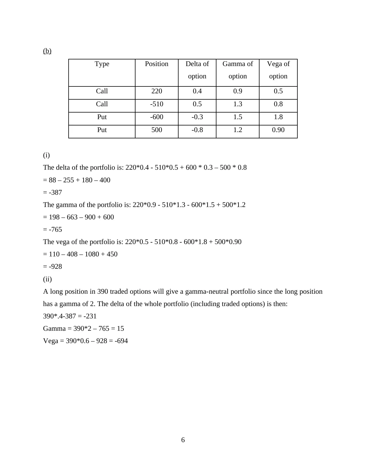
(b)
Type Position Delta of
option
Gamma of
option
Vega of
option
Call 220 0.4 0.9 0.5
Call -510 0.5 1.3 0.8
Put -600 -0.3 1.5 1.8
Put 500 -0.8 1.2 0.90
(i)
The delta of the portfolio is: 220*0.4 - 510*0.5 + 600 * 0.3 – 500 * 0.8
= 88 – 255 + 180 – 400
= -387
The gamma of the portfolio is: 220*0.9 - 510*1.3 - 600*1.5 + 500*1.2
= 198 – 663 – 900 + 600
= -765
The vega of the portfolio is: 220*0.5 - 510*0.8 - 600*1.8 + 500*0.90
= 110 – 408 – 1080 + 450
= -928
(ii)
A long position in 390 traded options will give a gamma-neutral portfolio since the long position
has a gamma of 2. The delta of the whole portfolio (including traded options) is then:
390*.4-387 = -231
Gamma = 390*2 – 765 = 15
Vega = 390*0.6 – 928 = -694
6
⊘ This is a preview!⊘
Do you want full access?
Subscribe today to unlock all pages.
Trusted by 1+ million students worldwide
(c).
A knock-in choice is latent option-contract as it only becomes active (or "knocks in") after
a certain cost level is achieved prior to expire. Knock-ins may be characterized either as a back
or an optional kind of obstacle. A barrier choice is a form of insurance wherein the compensation
is contingent on the value of the portfolio or whether it reaches a certain threshold. A barrier
choice is a form of insurance wherein the payoff is based mostly on value of the portfolio or even
if it reaches a certain cost over a certain time frame. Knock-in options are among 2 kinds of
barrier choices, with turn opportunities being another. A knock-in investor can purchase which is
only available if a certain cost is achieved. As a result, if the pricing has never been agreed
upon, the agreement ceases to exist. The knock-in alternative, on the other hand, is activated
when the asset value crosses a certain threshold. A knock-in choice arises only when the
underlying asset hits a boundary, whereas a knock-out choice begins to occur whenever the
underlying asset hits an obstacle. Barrier alternatives have cheaper insurance than vanilla
choices, owing to the increased risk of the choice being useless. Unless the fundamental is very
likely to strike the boundary, a seller might opt for the less expensive (in comparison to a similar
vanilla) barrier choice (Miura, Quadros, Gurumurthy and Ohtsuka, 2018).
Suspect a down-and-in call options with such a hurdle cost of $90 as well as a current
value of $100 is bought. The underlying asset is holding steady at $110, as well as the option has
a three-month expiration date. The alternative is created and will become a vanilla choice with
such a market price of $100 unless the volatility of the bond security hits $90. After that, even if
the asset value is traded beneath $90, the choice manager has the authority to acquire this at the
market price of $100. The alternative value is determined by this right which provide better
understanding of profit for the company. Even though the price of a security rises back below
$90, the option contract stays active until about the expiry date. The bottom expiration date
useless unless the asset value doesn't really fall far below intermediary price throughout the
contract terms life. The fact that the barrier has been breached does not guarantee a profit mostly
on trade so because fundamental must remain beneath $100, because after obstacle has been
triggered) in attempt for the alternative to be useful.
A back option, unlike an away option, only exists if the underlying crosses a barriers cost
that is greater than the current underlying's pricing. Presume a dealer buys one more a go call
option through an underlying value that is currently traded at $40 per percentage. The market
7
Paraphrase This Document
Need a fresh take? Get an instant paraphrase of this document with our AI Paraphraser
price including its out of call option contract is $50, with a hurdle of $55. The strike price of both
the back call futures contracts is $50, with a hurdle of $55. The choice deal ends worthless if the
asset value doesn't really exceed $55 within the duration of the agreement. The covered call will
become active and the investor would have been in the cash if the average investor rose to $55 or
higher (Golbabai, Nikan and Nikazad, 2019).
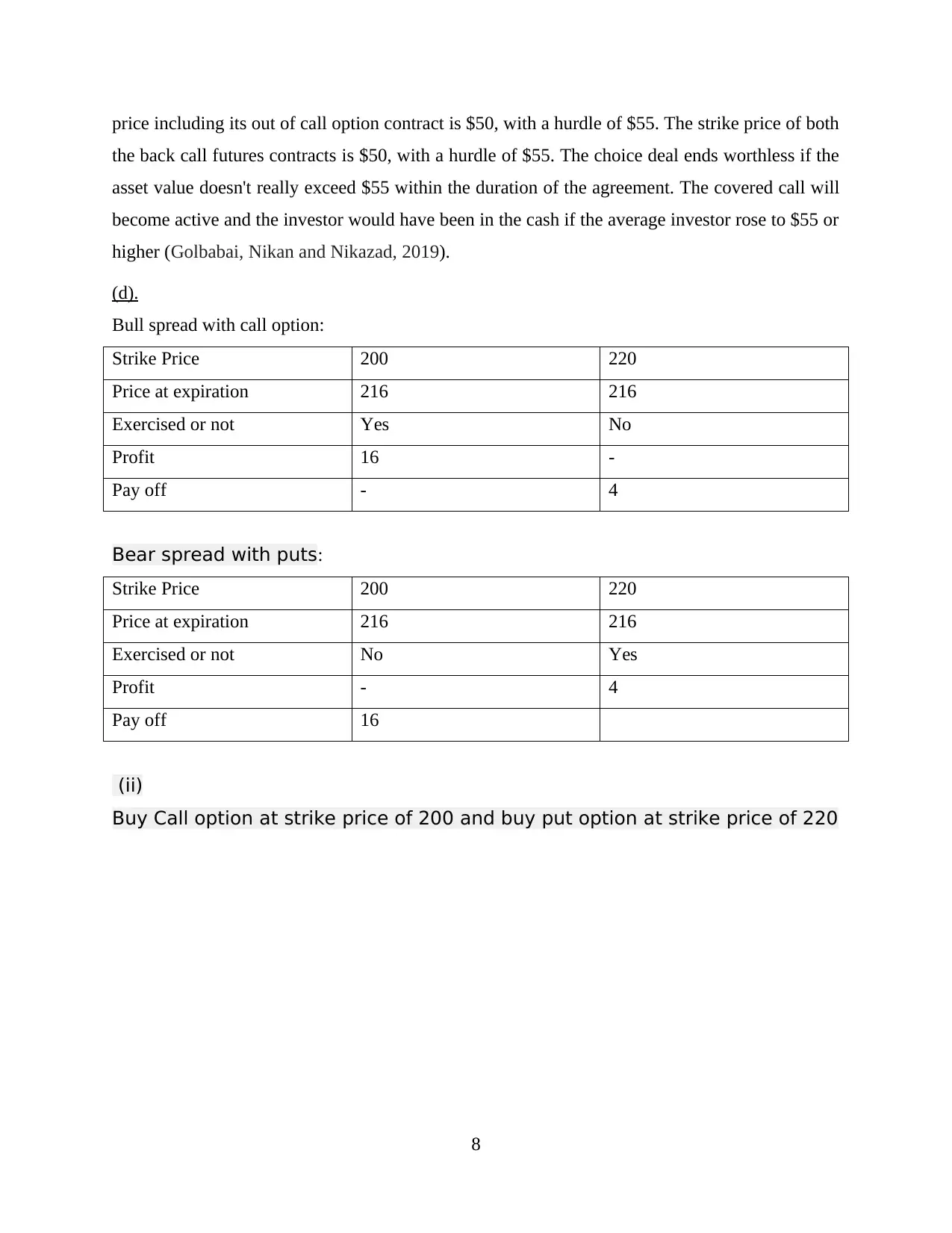
(d).
Bull spread with call option:
Strike Price 200 220
Price at expiration 216 216
Exercised or not Yes No
Profit 16 -
Pay off - 4
Bear spread with puts:
Strike Price 200 220
Price at expiration 216 216
Exercised or not No Yes
Profit - 4
Pay off 16
(ii)
Buy Call option at strike price of 200 and buy put option at strike price of 220
8
the back call futures contracts is $50, with a hurdle of $55. The choice deal ends worthless if the
asset value doesn't really exceed $55 within the duration of the agreement. The covered call will
become active and the investor would have been in the cash if the average investor rose to $55 or
higher (Golbabai, Nikan and Nikazad, 2019).
(d).
Bull spread with call option:
Strike Price 200 220
Price at expiration 216 216
Exercised or not Yes No
Profit 16 -
Pay off - 4
Bear spread with puts:
Strike Price 200 220
Price at expiration 216 216
Exercised or not No Yes
Profit - 4
Pay off 16
(ii)
Buy Call option at strike price of 200 and buy put option at strike price of 220
8
Question 3
Assumptions:
1. Random walk: The first premise, something that might recognize from other economic
projections, is that now the market price cannot be forecast uniformly and seems to be
entirely random. Price performs a so random walk, a moving characteristic often referred
it as Wave function or Brownian in astronomy. The very next movement will be down or
up at a certain moment, so company have no idea where it's going it will be.
2. Constant volatility: Volatility – the general magnitude of the movements, and in other
terms, how large or small movements they can anticipate – is one aspect we may
understand more about company's stock potential developments. Volatility is stable (does
not really change over time) and predictable in the Black-Scholes concept. Of course, in
the actual world, that presumption is extremely difficult (volatility is neither constant nor
known in advance). Simultaneously, volatility is among the model's variables that has the
greatest impact on the output price movement (Al–Zhour, Barfeie, Soleymani and Tohidi,
2019).
3. Normal distribution of return: Returns mostly on financial investment are traditionally
redistributed as a consequence of the randomness price path (assertion 1 above). The so-
called circular curve depicts the probability of subsequent percent change throughout the
stock's price over even a given timeframe, with smaller price movements close to just the
median having comparatively high probability and also more severe positively or
negatively cost increases being far less probable. When they get closer to the scales, the
percentages eventually decrease significantly. This is because of the connection
connecting distributions and prices, since returns are generally dispersed, prospective
asset values will be residuals are normally allocated at any specific moment in time.
In case if these assumptions are incorrect than option rise will show negative movement due to
which there can be adverse impact over the share price. Stock prices seldom exhibit lognormal
correlations, as Black-Scholes assumes. The distributions of the real world are distorted. As a
result of this disparity, the Black-Scholes model significantly under-priced or overpriced an
alternative. Traders who are acquainted with both the ramifications of the Black-Scholes models
may prefer to buy overvalued or short selling undervalued alternatives, causing them to losses.
To provide the most risk premium, investors must keep a close eye on price trends and market
9
⊘ This is a preview!⊘
Do you want full access?
Subscribe today to unlock all pages.
Trusted by 1+ million students worldwide
trends as a precautionary measure. Try to buy while volatility remains low (for example, over the
previous duration of the expected option holding period) but sell when it becomes high. In a
nutshell, market prices are believed to be absolute, without any connection to or dependence on
other industry trends or sections. The influence of the 2008–09 financial meltdown attributable to
just the housing market burst resulting in an overall financial meltdown, for instance, could be
counted for within the Black-Scholes modelling (or potentially any simulation theorem). A stock
with such a purchase of $100 as well as a distribution of $5 would drop to $95 on dividends ex-
date if all other variables remain constant. Option vendors take advantage of this opportunity by
selling short call/long futures contracts just before the expiration date and then squaring off the
roles on the expiration date, bringing in earnings. Traders who use Black-Scholes pricing must
be informed of these repercussions using a risk management strategy (De Staelen and Hendy,
2017).
10
Paraphrase This Document
Need a fresh take? Get an instant paraphrase of this document with our AI Paraphraser
References
Books and Journals:
Raimbourg, P. and Zimmermann, P., 2018, June. Is Normal Backwardation Normal? Valuing
Financial Futures with a Stochastic, Endogenous Index-Rate Covariance. In Valuing
Financial Futures with a Stochastic, Endogenous Index-Rate Covariance (June 3,
2018). Paris December 2018 Finance Meeting EUROFIDAI-AFFI.
Thirumagal, P.G. and SURESH, S., 2019. PAYOFF AND THE IMPACT OF VARIOUS
INVESTMENT ATTRIBUTES ON FREQUENCY OF INVESTMENT IN STOCK
INDEX FUTURES. International Journal of Mechanical and Production Engineering
Research and Development (IJMPERD) Vol, 8, pp.8-15.
Zanger, D.Z., 2018. Convergence of a least‐squares Monte Carlo algorithm for American option
pricing with dependent sample data. Mathematical Finance, 28(1), pp.447-479.
Ciorciari, J.D., 2019. The variable effectiveness of hedging strategies. International Relations of
the Asia-Pacific, 19(3), pp.523-555.
Haaland, T.R., Wright, J., Tufto, J. and Ratikainen, I.I., 2019. Short‐term insurance versus long‐
term bet‐hedging strategies as adaptations to variable environments. Evolution, 73(2),
pp.145-157.
Jia, L. and Chen, W., 2020. Knock-in options of an uncertain stock model with floating interest
rate. Chaos, Solitons & Fractals, 141, p.110324.
Miura, H., Quadros, R.M., Gurumurthy, C.B. and Ohtsuka, M., 2018. Easi-CRISPR for creating
knock-in and conditional knockout mouse models using long ssDNA donors. Nature
protocols, 13(1), p.195.
Golbabai, A., Nikan, O. and Nikazad, T., 2019. Numerical analysis of time fractional Black–
Scholes European option pricing model arising in financial market. Computational and
Applied Mathematics, 38(4), pp.1-24.
Al–Zhour, Z., Barfeie, M., Soleymani, F. and Tohidi, E., 2019. A computational method to price
with transaction costs under the nonlinear Black–Scholes model. Chaos, Solitons &
Fractals, 127, pp.291-301.
De Staelen, R.H. and Hendy, A.S., 2017. Numerically pricing double barrier options in a time-
fractional Black–Scholes model. Computers & Mathematics with Applications, 74(6),
pp.1166-1175.
11
1 out of 11
Related Documents


Your All-in-One AI-Powered Toolkit for Academic Success.
+13062052269
info@desklib.com
Available 24*7 on WhatsApp / Email
![[object Object]](/_next/static/media/star-bottom.7253800d.svg)
Unlock your academic potential
Copyright © 2020–2026 A2Z Services. All Rights Reserved. Developed and managed by ZUCOL.