Introduction to Biostatistics Assignment 2

This assignment covers topics such as calculating point estimate and confidence interval, appropriate charts to show distribution, hypothesis testing, contingency tables, sample size calculation and more in the context of biostatistics.

Running head: ASSIGNMENT TWO 0
introduction to biostatistics
Assignment 2
(NAME OF STUDENT)
university
Date of Submission

ASSIGNMENT TWO 2018 1
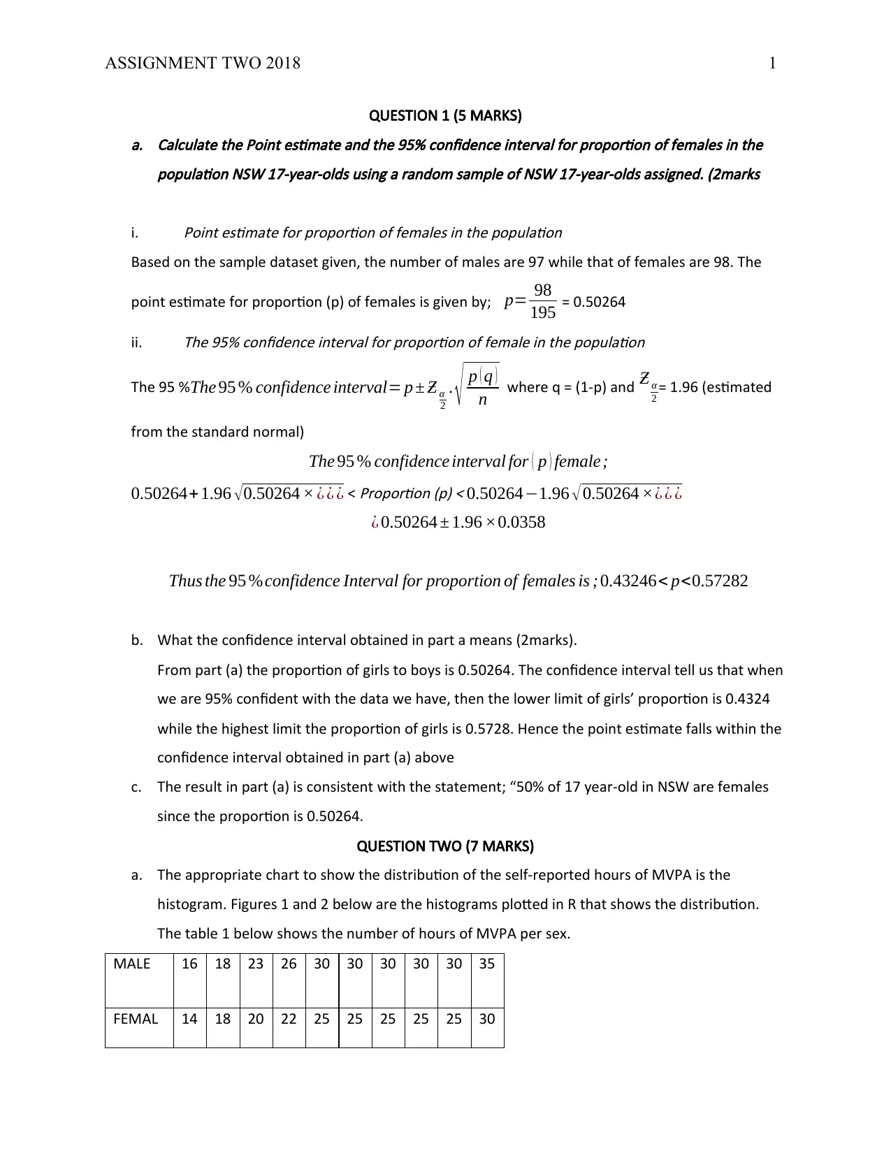
QUESTION 1 (5 MARKS)a. Calculate the Point estimate and the 95% confidence interval for proportion of females in the
population NSW 17-year-olds using a random sample of NSW 17-year-olds assigned. (2marks
i.
Point estimate for proportion of females in the population
Based on the sample dataset given, the number of males are 97 while that of females are 98. The
point estimate for proportion (p) of females is given by; p= 98
195 = 0.50264
ii.
The 95% confidence interval for proportion of female in the population
The 95 % The 95 % confidence interval= p ± Ƶ α
2
. √ p ( q )
n where q = (1-p) and Ƶ α
2 = 1.96 (estimated
from the standard normal)
The 95 % confidence interval for ( p ) female;
0.50264+ 1.96 √0.50264 × ¿ ¿ ¿ <
Proportion (p) < 0.50264−1.96 √ 0.50264 ׿ ¿ ¿
¿ 0.50264 ± 1.96 ×0.0358
Thus the 95 %confidence Interval for proportion of females is ;0.43246< p<0.57282
b. What the confidence interval obtained in part a means (2marks).
From part (a) the proportion of girls to boys is 0.50264. The confidence interval tell us that when
we are 95% confident with the data we have, then the lower limit of girls’ proportion is 0.4324
while the highest limit the proportion of girls is 0.5728. Hence the point estimate falls within the
confidence interval obtained in part (a) above
c. The result in part (a) is consistent with the statement; “50% of 17 year-old in NSW are females
since the proportion is 0.50264.
QUESTION TWO (7 MARKS)
a. The appropriate chart to show the distribution of the self-reported hours of MVPA is the
histogram. Figures 1 and 2 below are the histograms plotted in R that shows the distribution.
The table 1 below shows the number of hours of MVPA per sex.
MALE 16 18 23 26 30 30 30 30 30 35
FEMAL 14 18 20 22 25 25 25 25 25 30

ASSIGNMENT TWO 2018 2
E
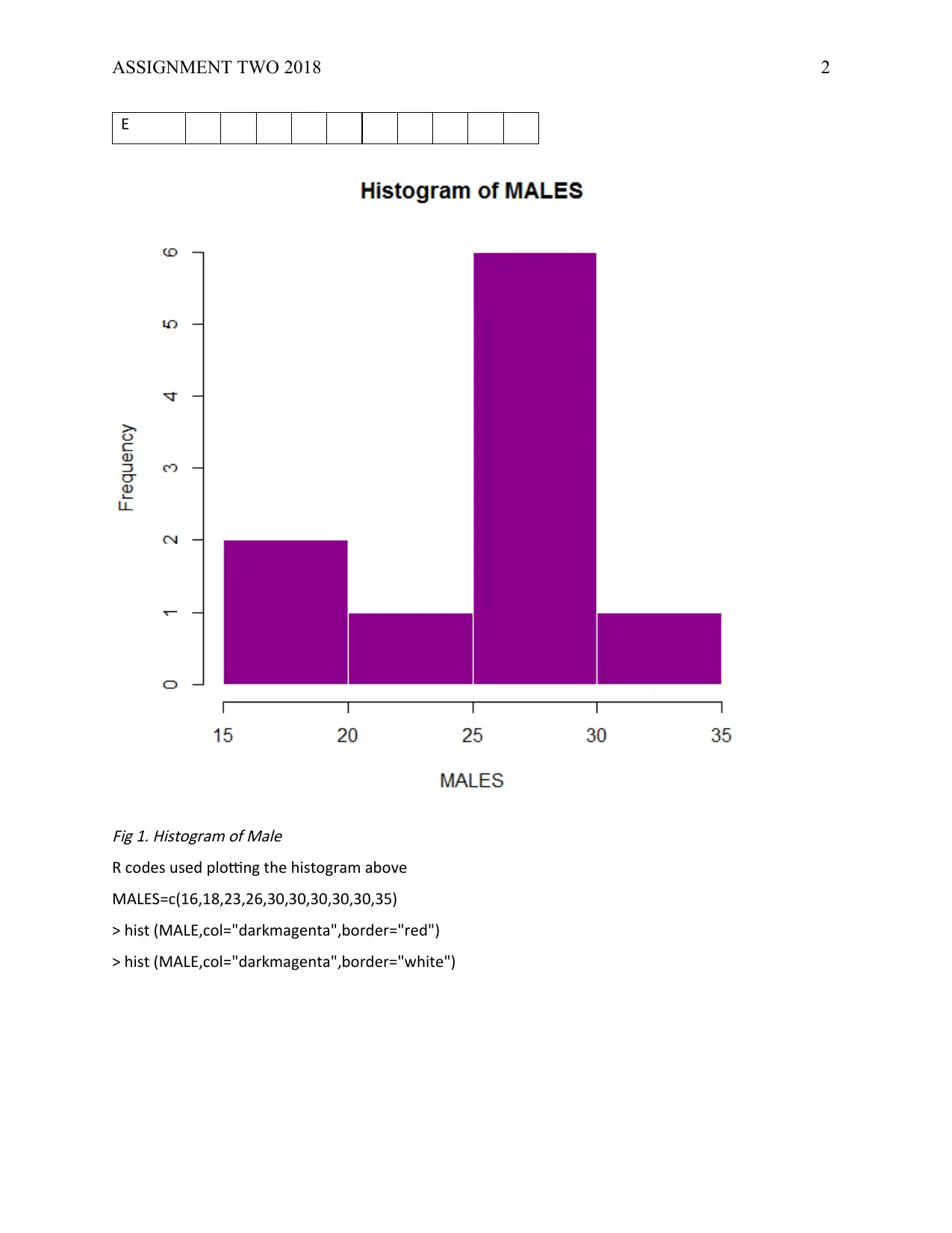
Fig 1. Histogram of Male
R codes used plotting the histogram above
MALES=c(16,18,23,26,30,30,30,30,30,35)
> hist (MALE,col="darkmagenta",border="red")
> hist (MALE,col="darkmagenta",border="white")

ASSIGNMENT TWO 2018 3
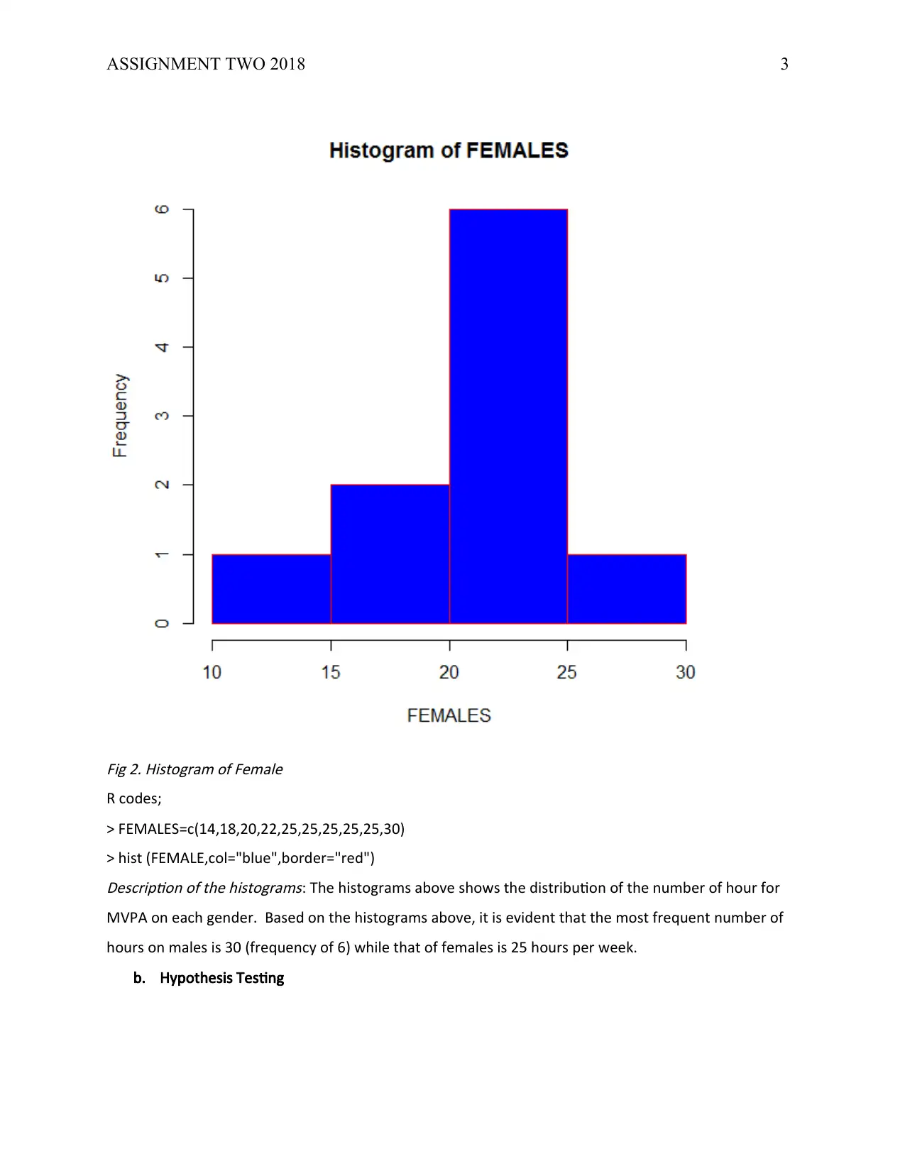
Fig 2. Histogram of Female
R codes;
> FEMALES=c(14,18,20,22,25,25,25,25,25,30)
> hist (FEMALE,col="blue",border="red")Description of the histograms: The histograms above shows the distribution of the number of hour for
MVPA on each gender. Based on the histograms above, it is evident that the most frequent number of
hours on males is 30 (frequency of 6) while that of females is 25 hours per week.
b. Hypothesis Testing

ASSIGNMENT TWO 2018 4
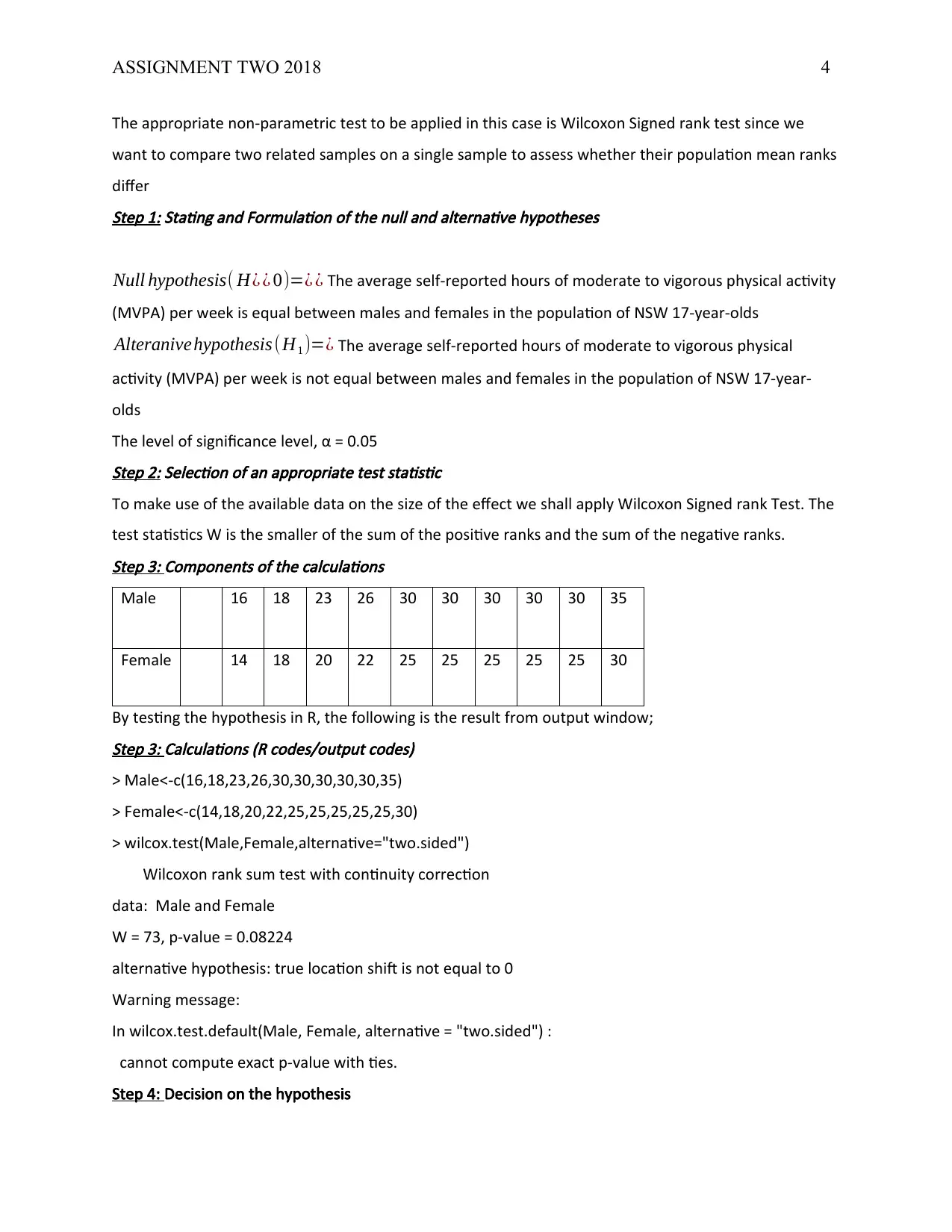
The appropriate non-parametric test to be applied in this case is Wilcoxon Signed rank test since we
want to compare two related samples on a single sample to assess whether their population mean ranks
differStep 1: Stating and Formulation of the null and alternative hypotheses
Null hypothesis( H¿ ¿ 0)=¿ ¿ The average self-reported hours of moderate to vigorous physical activity
(MVPA) per week is equal between males and females in the population of NSW 17-year-olds
Alteranivehypothesis (H1 )=¿ The average self-reported hours of moderate to vigorous physical
activity (MVPA) per week is not equal between males and females in the population of NSW 17-year-
olds
The level of significance level, α = 0.05Step 2: Selection of an appropriate test statistic
To make use of the available data on the size of the effect we shall apply Wilcoxon Signed rank Test. The
test statistics W is the smaller of the sum of the positive ranks and the sum of the negative ranks.Step 3: Components of the calculations
Male 16 18 23 26 30 30 30 30 30 35
Female 14 18 20 22 25 25 25 25 25 30
By testing the hypothesis in R, the following is the result from output window;Step 3: Calculations (R codes/output codes)
> Male<-c(16,18,23,26,30,30,30,30,30,35)
> Female<-c(14,18,20,22,25,25,25,25,25,30)
> wilcox.test(Male,Female,alternative="two.sided")
Wilcoxon rank sum test with continuity correction
data: Male and Female
W = 73, p-value = 0.08224
alternative hypothesis: true location shift is not equal to 0
Warning message:
In wilcox.test.default(Male, Female, alternative = "two.sided") :
cannot compute exact p-value with ties.
Step 4: Decision on the hypothesis

ASSIGNMENT TWO 2018 5
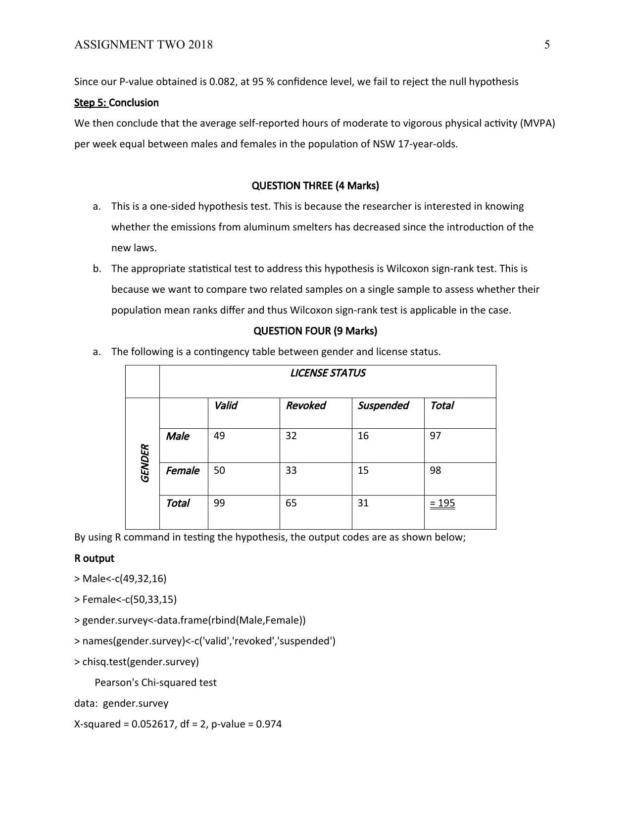
Since our P-value obtained is 0.082, at 95 % confidence level, we fail to reject the null hypothesis
Step 5: Conclusion
We then conclude that the average self-reported hours of moderate to vigorous physical activity (MVPA)
per week equal between males and females in the population of NSW 17-year-olds.
QUESTION THREE (4 Marks)
a. This is a one-sided hypothesis test. This is because the researcher is interested in knowing
whether the emissions from aluminum smelters has decreased since the introduction of the
new laws.
b. The appropriate statistical test to address this hypothesis is Wilcoxon sign-rank test. This is
because we want to compare two related samples on a single sample to assess whether their
population mean ranks differ and thus Wilcoxon sign-rank test is applicable in the case.
QUESTION FOUR (9 Marks)
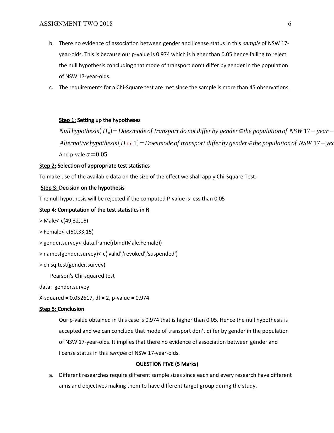
a. The following is a contingency table between gender and license status.
LICENSE STATUS
GENDER
Valid
Revoked Suspended Total
Male 49 32 16 97
Female 50 33 15 98
Total 99 65 31 = 195
By using R command in testing the hypothesis, the output codes are as shown below;
R output
> Male<-c(49,32,16)
> Female<-c(50,33,15)
> gender.survey<-data.frame(rbind(Male,Female))
> names(gender.survey)<-c('valid','revoked','suspended')
> chisq.test(gender.survey)
Pearson's Chi-squared test
data: gender.survey
X-squared = 0.052617, df = 2, p-value = 0.974

ASSIGNMENT TWO 2018 6
b. There no evidence of association between gender and license status in this
sample of NSW 17-
year-olds. This is because our p-value is 0.974 which is higher than 0.05 hence failing to reject
the null hypothesis concluding that mode of transport don’t differ by gender in the population
of NSW 17-year-olds.
c. The requirements for a Chi-Square test are met since the sample is more than 45 observations.
Step 1: Setting up the hypotheses
Null hypothesis( H0)=Doesmode of transport do not differ by gender ∈the population of NSW 17− year−
Alternative hypothesis (H ¿¿ 1)=Doesmode of transport differ by gender ∈the population of NSW 17− yea
And p-vale α=0.05
Step 2: Selection of appropriate test statistics
To make use of the available data on the size of the effect we shall apply Chi-Square Test.
Step 3: Decision on the hypothesis
The null hypothesis will be rejected if the computed P-value is less than 0.05
Step 4: Computation of the test statistics in R
> Male<-c(49,32,16)
> Female<-c(50,33,15)
> gender.survey<-data.frame(rbind(Male,Female))
> names(gender.survey)<-c('valid','revoked','suspended')
> chisq.test(gender.survey)
Pearson's Chi-squared test
data: gender.survey
X-squared = 0.052617, df = 2, p-value = 0.974
Step 5: Conclusion
Our p-value obtained in this case is 0.974 that is higher than 0.05. Hence the null hypothesis is
accepted and we can conclude that mode of transport don’t differ by gender in the population
of NSW 17-year-olds. It implies that there no evidence of association between gender and
license status in this
sample of NSW 17-year-olds.
QUESTION FIVE (5 Marks)
a. Different researches require different sample sizes since each and every research have different
aims and objectives making them to have different target group during the study.

ASSIGNMENT TWO 2018 7
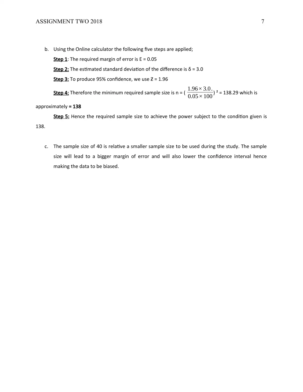
b. Using the Online calculator the following five steps are applied;
Step 1: The required margin of error is E = 0.05
Step 2: The estimated standard deviation of the difference is δ = 3.0
Step 3: To produce 95% confidence, we use Ƶ = 1.96
Step 4: Therefore the minimum required sample size is n = ( 1.96× 3.0 .
0.05× 100 ) ² = 138.29 which is
approximately = 138
Step 5: Hence the required sample size to achieve the power subject to the condition given is
138.
c. The sample size of 40 is relative a smaller sample size to be used during the study. The sample
size will lead to a bigger margin of error and will also lower the confidence interval hence
making the data to be biased.