Data Analysis of Sample 107
VerifiedAdded on 2020/05/16
|16
|2113
|29
AI Summary
This assignment involves analyzing a dataset from Sample 107. The dataset explores various aspects such as preferences for machine A or B, casino profit, and support for a proposed change. It includes descriptive statistics presented in tables and visualized using histograms and scatter plots. The analysis aims to uncover patterns and insights within the sample data.
Contribute Materials
Your contribution can guide someone’s learning journey. Share your
documents today.

RUNNING HEADER: Bus105 computing assignment 1
Bus105 computing assignment
Name:Aanchal ANEJA
Student number:11600869
Allocated sample: 107
Bus105 computing assignment
Name:Aanchal ANEJA
Student number:11600869
Allocated sample: 107
Secure Best Marks with AI Grader
Need help grading? Try our AI Grader for instant feedback on your assignments.
Bus105 computing assignment 2
Introduction
Statistical analysis is an important component for business intelligence. Statistical analysis
assists in scrutinizing every data sample in data sets from which samples are drawn (Chen et
al., 2012, p.16). The process of statistical analysis entail description of the nature of data that
is chosen for analysis, investigating the relationships of data in the primary population,
creation of models to assist in summarizing the comprehension of how data relates to the
primary population, proving the data validity and employing analytics that is predictive to run
the different states which will assist in upcoming events.
Section 1
* Datasets
A data set is a collection of discrete items that contain related data which can be accessed
exclusively or in combination or managed as a complete unit (Johnson &Wichen, 2014, p.5).
Datasets are organized into some type of data structure such as a collection of business data.
*Variable
On the other hand, a variable is a number, quantity or a characteristic which either increase or
decreases over time (Johnson & Wichen, 2014, p.5). Moreover, it takes different values in
different situations.
*How to summarize a variable and the relationship between
Based on its nature, a variable can be summarized in various ways. A variable can either be
discrete or continuous. Discrete variables can be summarized using frequency distribution
tables and graphical summaries such as bar charts, histograms. On the other hand, continuous
variables can be summarized using descriptive statistics which entail the means, standard
deviations, variances, standard errors, range, mode, and median among others.
Bus105 computing assignment 3
Consideration of two variables entails the nature of the variable. That is, whether the variable
is categorical or quantitative. When comparing the relationship between two variables, which
are categorical in nature, the analysis is made on the relationship during an assessment of
conditional probabilities. Furthermore a graphical representation is made of the data using
contingency tables. Such categorical variables can include class standings and gender. When
both variables are quantitative, the analysis is made on how one of the variables, the response
variable, changes with respect to the changes of the other variable, the explanatory variable.
To show the relationship graphically, scatter plots are used. The last scenario is when one of
the variables is categorical while the other is quantitative. A good example is between gender
and height. In this scenario, the comparison is best made using side-by-side box plots which
show whichever similarities or differences in the center and the changeability of the variable
which is quantitative across the categories.
*why is important to be able to find patterns in a dataset using a computer
Finding patterns in a dataset is very vital in numerous ways. For starters, the pattern can be
used to find inherent regularities in a data set. On the other hand, the pattern can be used as a
foundation for various essential tasks. Such tasks include correlation, association, causality
analysis, mining sequential, pattern analysis in stream and time series data, structural
patterns, for categorization through discriminative analysis that is based on patterns, and
cluster analysis through subspace clustering that is based on patterns. As a result, pattern
finding in a dataset using computers has a broad application in cross-marketing, catalog
design, market basket analysis, web log analysis, sale campaign analysis, and biological
sequence analysis.
Bus105 computing assignment 4
Section 2
a) Sample 107
10,000 20,000 30,000 40,000 50,000 60,000
$8,000
$10,000
$12,000
$14,000
$16,000
$18,000
$20,000
$22,000
f(x) = − 0.158496496105284 x + 19253.0627207946
Distance travelled
Selling price
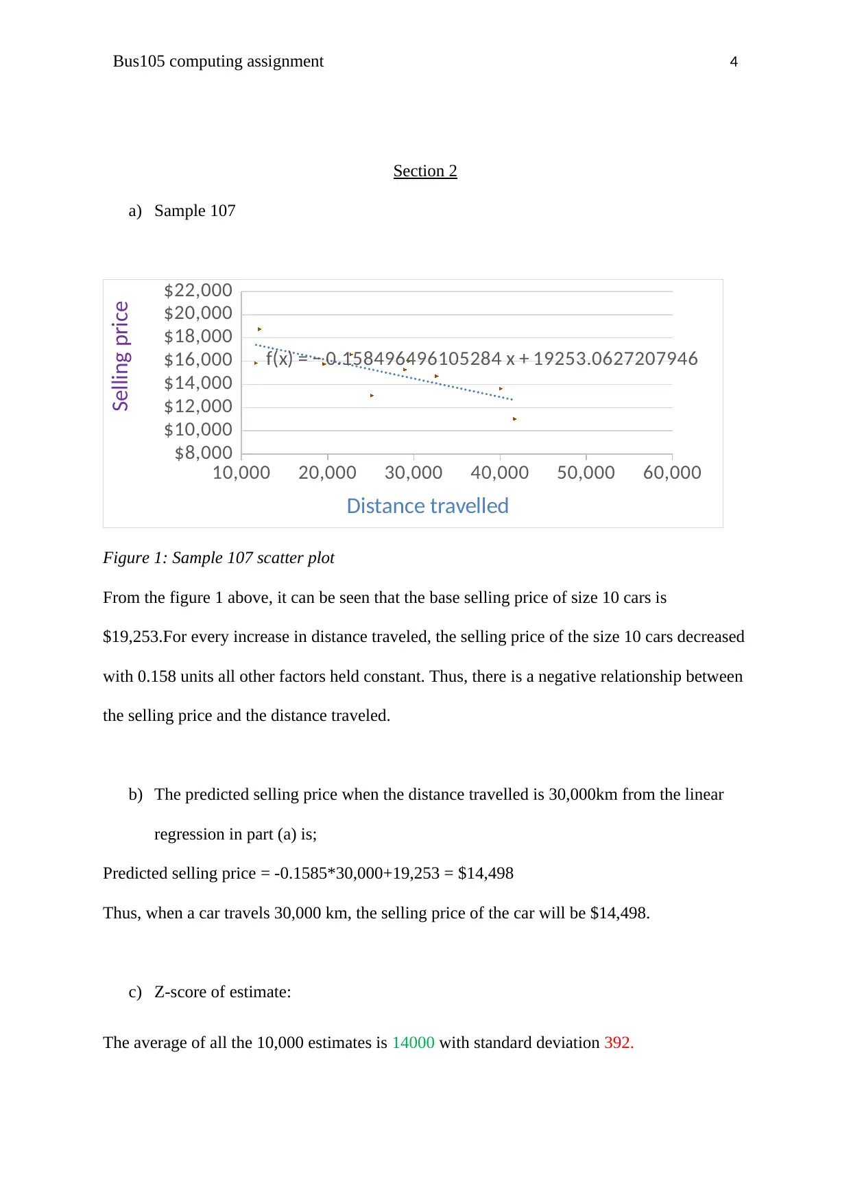
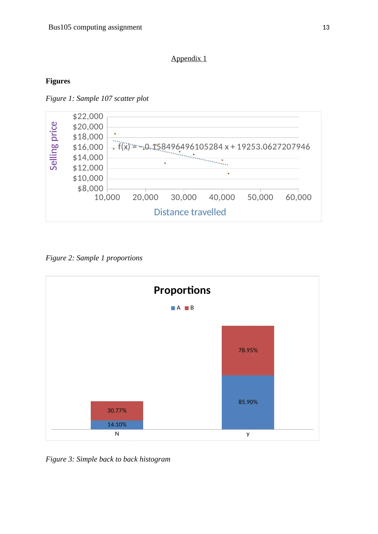
Figure 1: Sample 107 scatter plot
From the figure 1 above, it can be seen that the base selling price of size 10 cars is
$19,253.For every increase in distance traveled, the selling price of the size 10 cars decreased
with 0.158 units all other factors held constant. Thus, there is a negative relationship between
the selling price and the distance traveled.
b) The predicted selling price when the distance travelled is 30,000km from the linear
regression in part (a) is;
Predicted selling price = -0.1585*30,000+19,253 = $14,498
Thus, when a car travels 30,000 km, the selling price of the car will be $14,498.
c) Z-score of estimate:
The average of all the 10,000 estimates is 14000 with standard deviation 392.
Section 2
a) Sample 107
10,000 20,000 30,000 40,000 50,000 60,000
$8,000
$10,000
$12,000
$14,000
$16,000
$18,000
$20,000
$22,000
f(x) = − 0.158496496105284 x + 19253.0627207946
Distance travelled
Selling price
Figure 1: Sample 107 scatter plot
From the figure 1 above, it can be seen that the base selling price of size 10 cars is
$19,253.For every increase in distance traveled, the selling price of the size 10 cars decreased
with 0.158 units all other factors held constant. Thus, there is a negative relationship between
the selling price and the distance traveled.
b) The predicted selling price when the distance travelled is 30,000km from the linear
regression in part (a) is;
Predicted selling price = -0.1585*30,000+19,253 = $14,498
Thus, when a car travels 30,000 km, the selling price of the car will be $14,498.
c) Z-score of estimate:
The average of all the 10,000 estimates is 14000 with standard deviation 392.
Secure Best Marks with AI Grader
Need help grading? Try our AI Grader for instant feedback on your assignments.
Bus105 computing assignment 5
So the z-score for sample 1 estimate is (14,498-14000)/392= 1.265
d) P (z-score);
Using wolframalpha.com P(Z<1.265)=0.8972
e) Rank;
So if you compare sample 107 to the 10,000 samples then
Predicted rank = P(Z<z-score)*10000=0.8972*10,000=8,972
Thus, the estimate would rank at 8,972 out of 10,000.
Section 3
a)
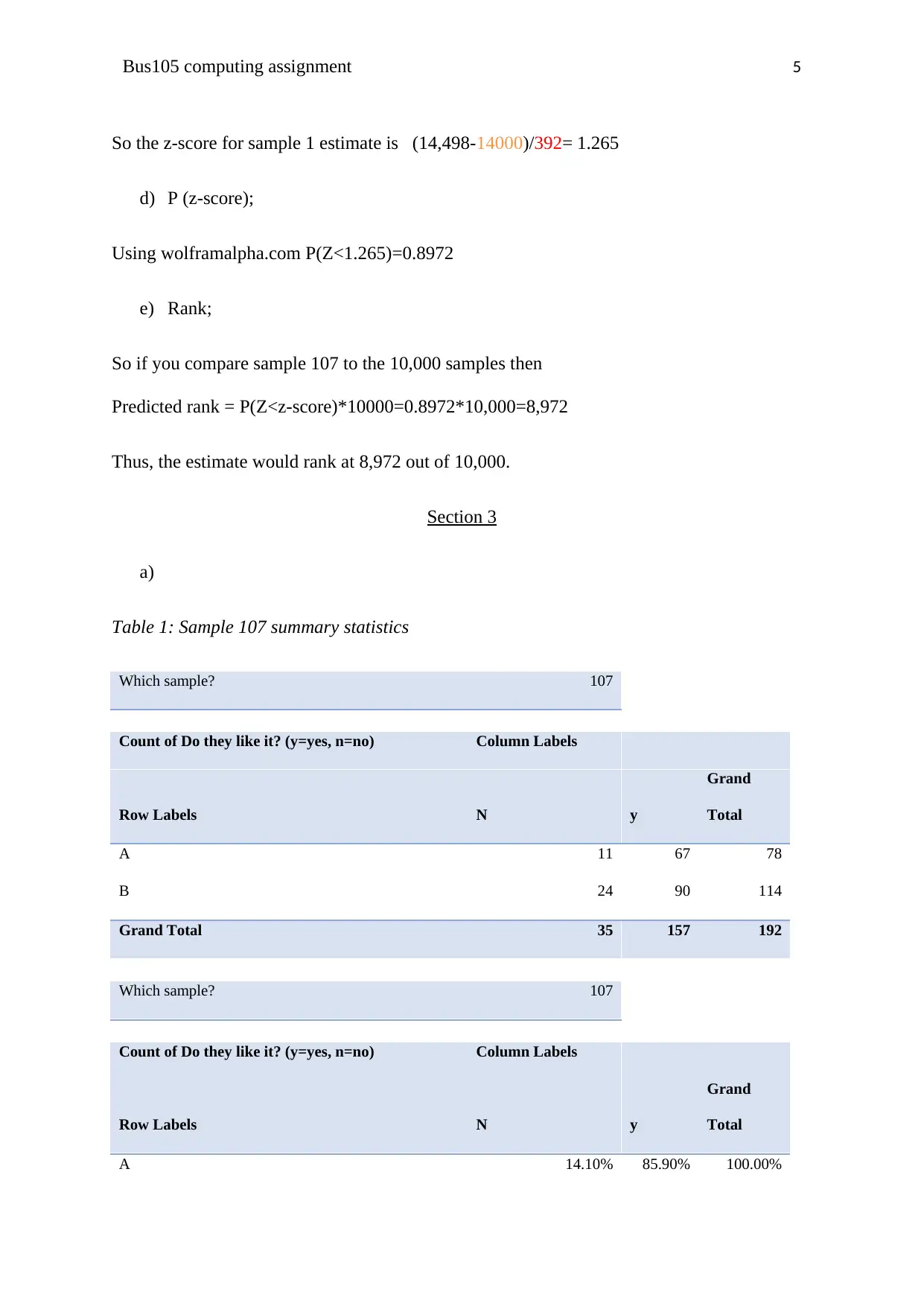
Table 1: Sample 107 summary statistics
Which sample? 107
Count of Do they like it? (y=yes, n=no) Column Labels
Row Labels N y
Grand
Total
A 11 67 78
B 24 90 114
Grand Total 35 157 192
Which sample? 107
Count of Do they like it? (y=yes, n=no) Column Labels
Row Labels N y
Grand
Total
A 14.10% 85.90% 100.00%
So the z-score for sample 1 estimate is (14,498-14000)/392= 1.265
d) P (z-score);
Using wolframalpha.com P(Z<1.265)=0.8972
e) Rank;
So if you compare sample 107 to the 10,000 samples then
Predicted rank = P(Z<z-score)*10000=0.8972*10,000=8,972
Thus, the estimate would rank at 8,972 out of 10,000.
Section 3
a)
Table 1: Sample 107 summary statistics
Which sample? 107
Count of Do they like it? (y=yes, n=no) Column Labels
Row Labels N y
Grand
Total
A 11 67 78
B 24 90 114
Grand Total 35 157 192
Which sample? 107
Count of Do they like it? (y=yes, n=no) Column Labels
Row Labels N y
Grand
Total
A 14.10% 85.90% 100.00%
Bus105 computing assignment 6
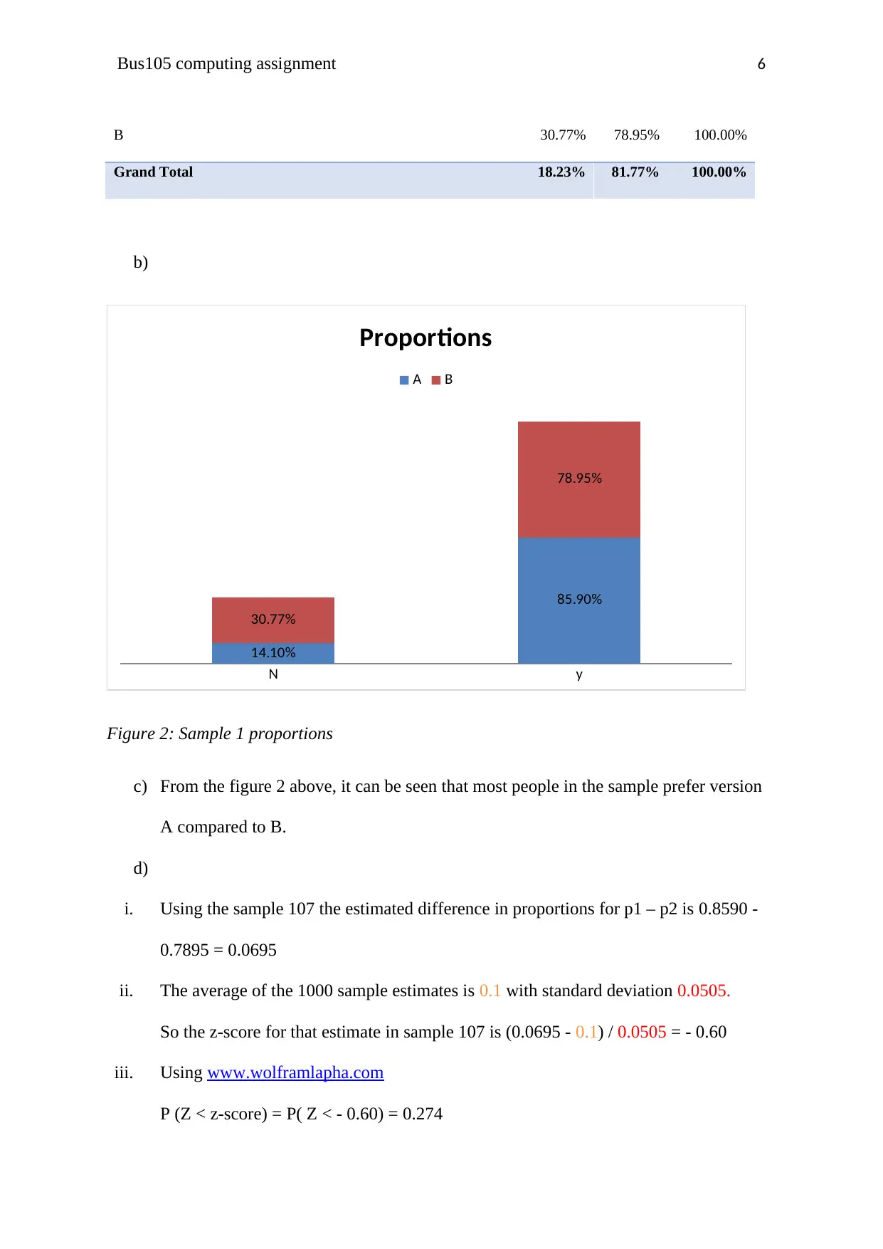
B 30.77% 78.95% 100.00%
Grand Total 18.23% 81.77% 100.00%
b)
N y
14.10%
85.90%
30.77%
78.95%
Proportions
A B
Figure 2: Sample 1 proportions
c) From the figure 2 above, it can be seen that most people in the sample prefer version
A compared to B.
d)
i. Using the sample 107 the estimated difference in proportions for p1 – p2 is 0.8590 -
0.7895 = 0.0695
ii. The average of the 1000 sample estimates is 0.1 with standard deviation 0.0505.
So the z-score for that estimate in sample 107 is (0.0695 - 0.1) / 0.0505 = - 0.60
iii. Using www.wolframlapha.com
P (Z < z-score) = P( Z < - 0.60) = 0.274
Bus105 computing assignment 7
iv. So when you compare sample 107 to the 1000 other samples you predict the rank to
be
0.274 * 1000 = 274
e) To test the claim that there is a difference in proportions, the following hypothesis was
formulated:
i. Hypothesis;
H0: There is no difference between the proportions, p1 = p2
H1: There is a difference between the proportions, p1 ≠p2
ii. The resultant p-value from www.epitools.com is 0.2205.
iii. Since the p-value is greater than 0.05, we do not reject the H0.
iv. Thus, there is strong evidence which shows that there is no difference between the
sample proportions.
Section 4
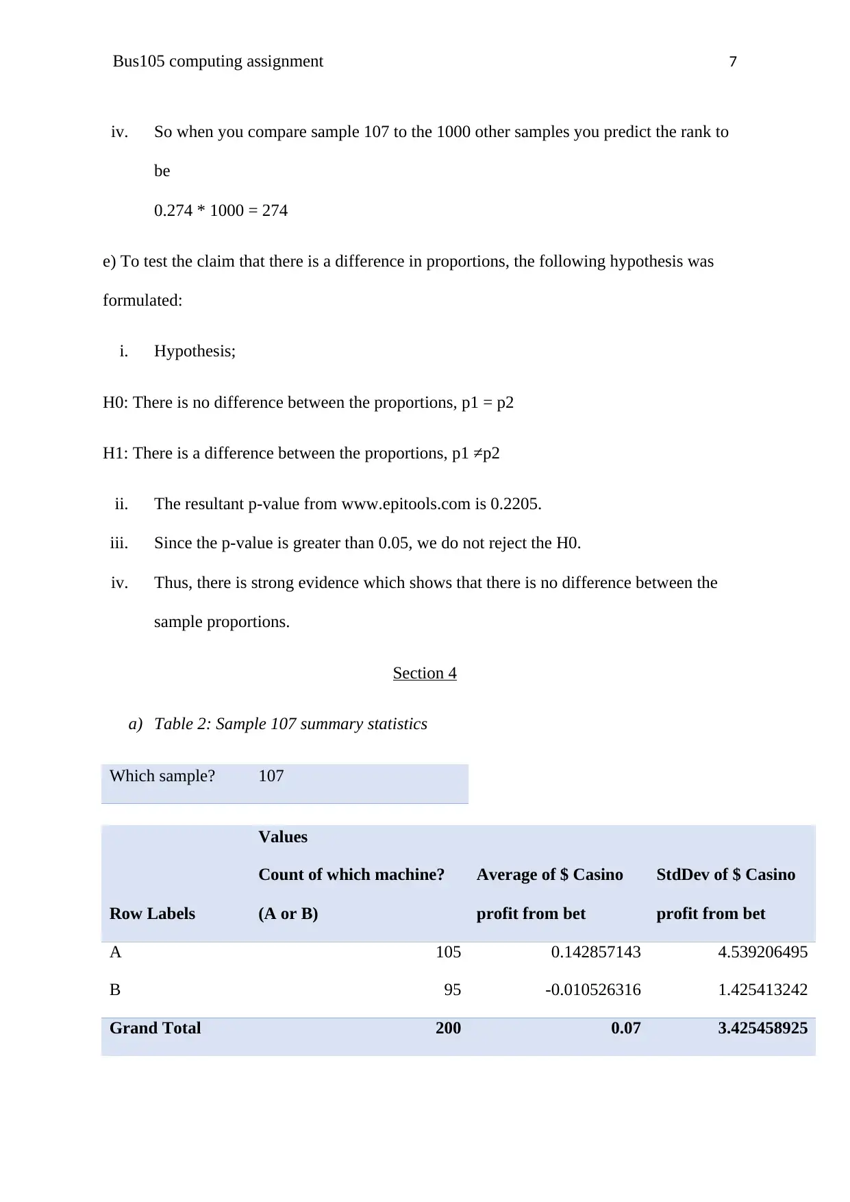
a) Table 2: Sample 107 summary statistics
Which sample? 107
Values
Row Labels
Count of which machine?
(A or B)
Average of $ Casino
profit from bet
StdDev of $ Casino
profit from bet
A 105 0.142857143 4.539206495
B 95 -0.010526316 1.425413242
Grand Total 200 0.07 3.425458925
iv. So when you compare sample 107 to the 1000 other samples you predict the rank to
be
0.274 * 1000 = 274
e) To test the claim that there is a difference in proportions, the following hypothesis was
formulated:
i. Hypothesis;
H0: There is no difference between the proportions, p1 = p2
H1: There is a difference between the proportions, p1 ≠p2
ii. The resultant p-value from www.epitools.com is 0.2205.
iii. Since the p-value is greater than 0.05, we do not reject the H0.
iv. Thus, there is strong evidence which shows that there is no difference between the
sample proportions.
Section 4
a) Table 2: Sample 107 summary statistics
Which sample? 107
Values
Row Labels
Count of which machine?
(A or B)
Average of $ Casino
profit from bet
StdDev of $ Casino
profit from bet
A 105 0.142857143 4.539206495
B 95 -0.010526316 1.425413242
Grand Total 200 0.07 3.425458925
Paraphrase This Document
Need a fresh take? Get an instant paraphrase of this document with our AI Paraphraser
Bus105 computing assignment 8
b)
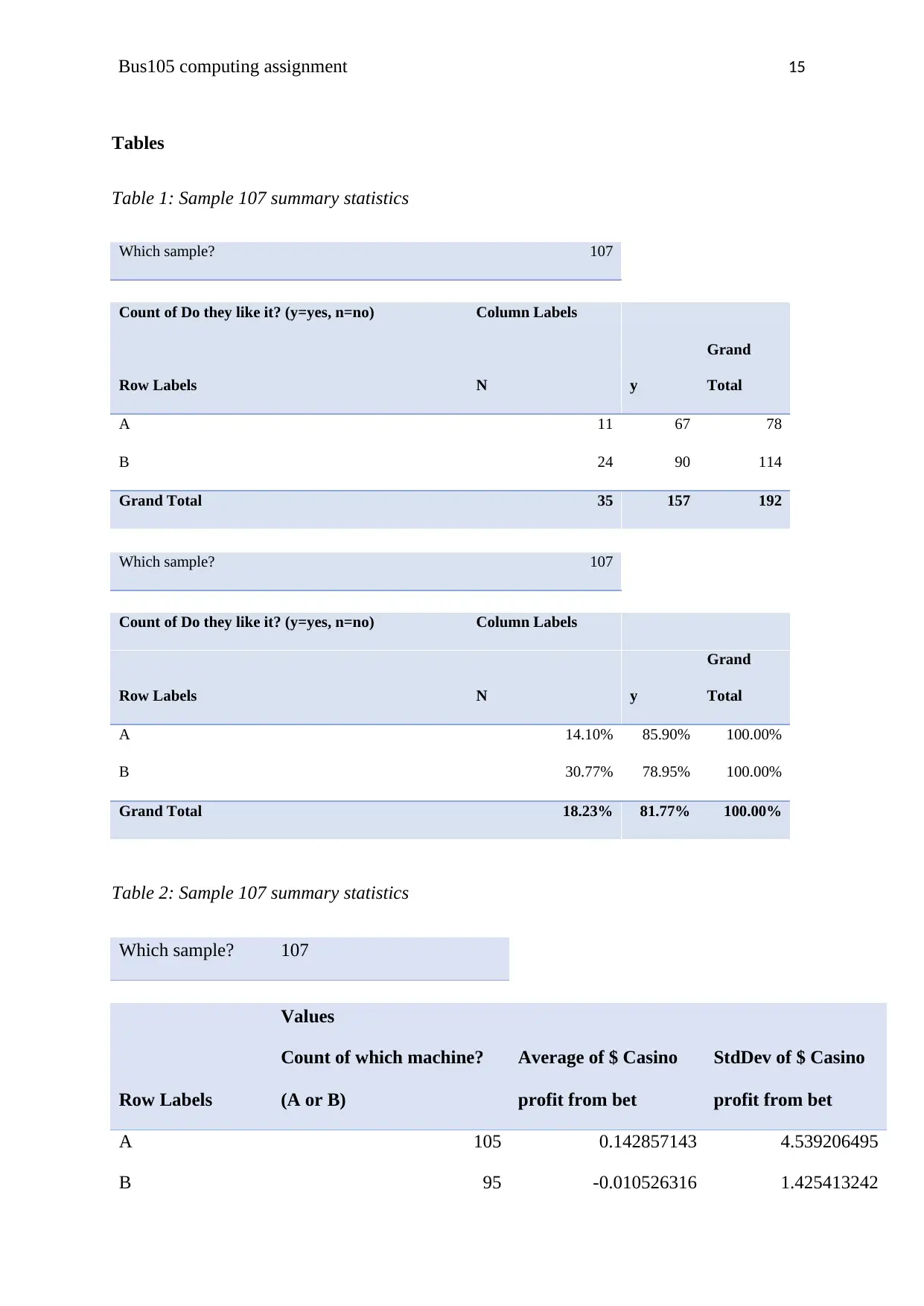
From the table 2 above, it can be seen that machine A had an average profit of 0.14 while
machine B made a loss averaging 0.01. On the other hand, the profits from machine A had a
large spread of 4.54 while machine B had a lower spread of 1.42 compared to machine A.
c)
i. So for sample 107 the estimate of the difference in the population means is the
difference in the sample means; x1−x2= 0.143 - - 0.011 = 0.154
ii. The average of the 2000 sample estimates is 0.4 with standard deviation 0.46 so the
z-score of the sample 100 estimate is = (0.154 - 0.4) / 0.46 = - 0.535
iii. Using wolframalpha.com P (Z < z-score) = P (Z < - 0.535) = 0.296
iv. So if you compare the sample estimate 700 to the 2000 other sample estimates you
expect it to have rank 1000 * 0.295 = 296
d) To test the claim that there is a difference in means, the following hypothesis was
formulated:
i. H0: There is no difference in the sample proportions p1 = p2
H1: There is a difference in the sample proportions p1 ≠p2
ii. The resultant p-value from www.epitools.com is 0.5035.
iii. Since the p-value is greater than 0.05, we do not reject the H0.
iv. Thus, there is strong evidence which shows that there is no difference between
proportions.
b)
From the table 2 above, it can be seen that machine A had an average profit of 0.14 while
machine B made a loss averaging 0.01. On the other hand, the profits from machine A had a
large spread of 4.54 while machine B had a lower spread of 1.42 compared to machine A.
c)
i. So for sample 107 the estimate of the difference in the population means is the
difference in the sample means; x1−x2= 0.143 - - 0.011 = 0.154
ii. The average of the 2000 sample estimates is 0.4 with standard deviation 0.46 so the
z-score of the sample 100 estimate is = (0.154 - 0.4) / 0.46 = - 0.535
iii. Using wolframalpha.com P (Z < z-score) = P (Z < - 0.535) = 0.296
iv. So if you compare the sample estimate 700 to the 2000 other sample estimates you
expect it to have rank 1000 * 0.295 = 296
d) To test the claim that there is a difference in means, the following hypothesis was
formulated:
i. H0: There is no difference in the sample proportions p1 = p2
H1: There is a difference in the sample proportions p1 ≠p2
ii. The resultant p-value from www.epitools.com is 0.5035.
iii. Since the p-value is greater than 0.05, we do not reject the H0.
iv. Thus, there is strong evidence which shows that there is no difference between
proportions.
Bus105 computing assignment 9
Section 5
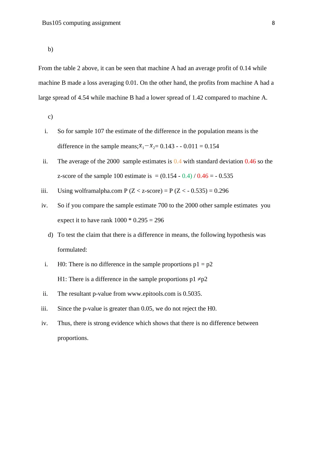
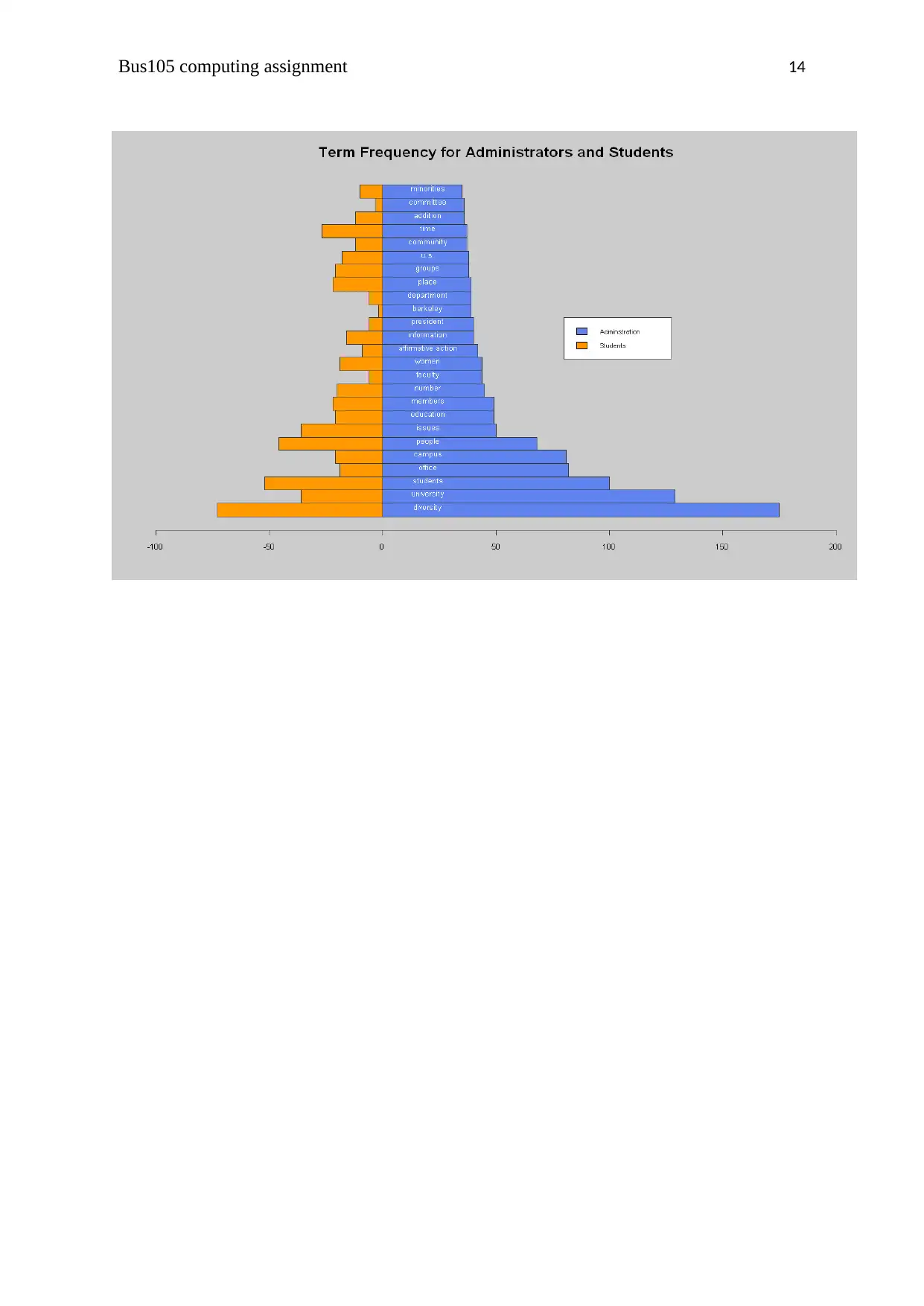
Figure 3: Simple back to back histogram
*Description of each variable
The figure above is a back to back histogram showing the frequency of terms used by
students and the administration. The x-axis is a dummy variable that shows whether the
variable is a student or n administrator. The x-axis answers the question, "is the participant a
student or in administration?" Thus, it is categorical n nature.
*Relationship between the variables
The y-axis is the frequency of the terms that are used by either the administration or the
students. It answers the question, "How often do you use the following term?" Thus, it is
quantitative in nature.
Section 5
Figure 3: Simple back to back histogram
*Description of each variable
The figure above is a back to back histogram showing the frequency of terms used by
students and the administration. The x-axis is a dummy variable that shows whether the
variable is a student or n administrator. The x-axis answers the question, "is the participant a
student or in administration?" Thus, it is categorical n nature.
*Relationship between the variables
The y-axis is the frequency of the terms that are used by either the administration or the
students. It answers the question, "How often do you use the following term?" Thus, it is
quantitative in nature.
Bus105 computing assignment 10
Based on the bars on the right side of the back to back histogram, one can see a curved
pattern. On the left side, a jagged pattern is observed. Thus, it is evident that the terms used
by the students and the administration staff do not quite match in frequency. However, long
bars are at the bottom while the short bars are t the top thereby implying that the
discrepancies are not very big.
*Would a business be able to use back to back histogram?
No. A business would not use a back to back histogram. Though back to back histograms are
visually strong and can compare to normal curves, they cannot read exact values of variables
since the data is grouped into categories. As a result, it will be difficult to compare two data
sets.
Section 6
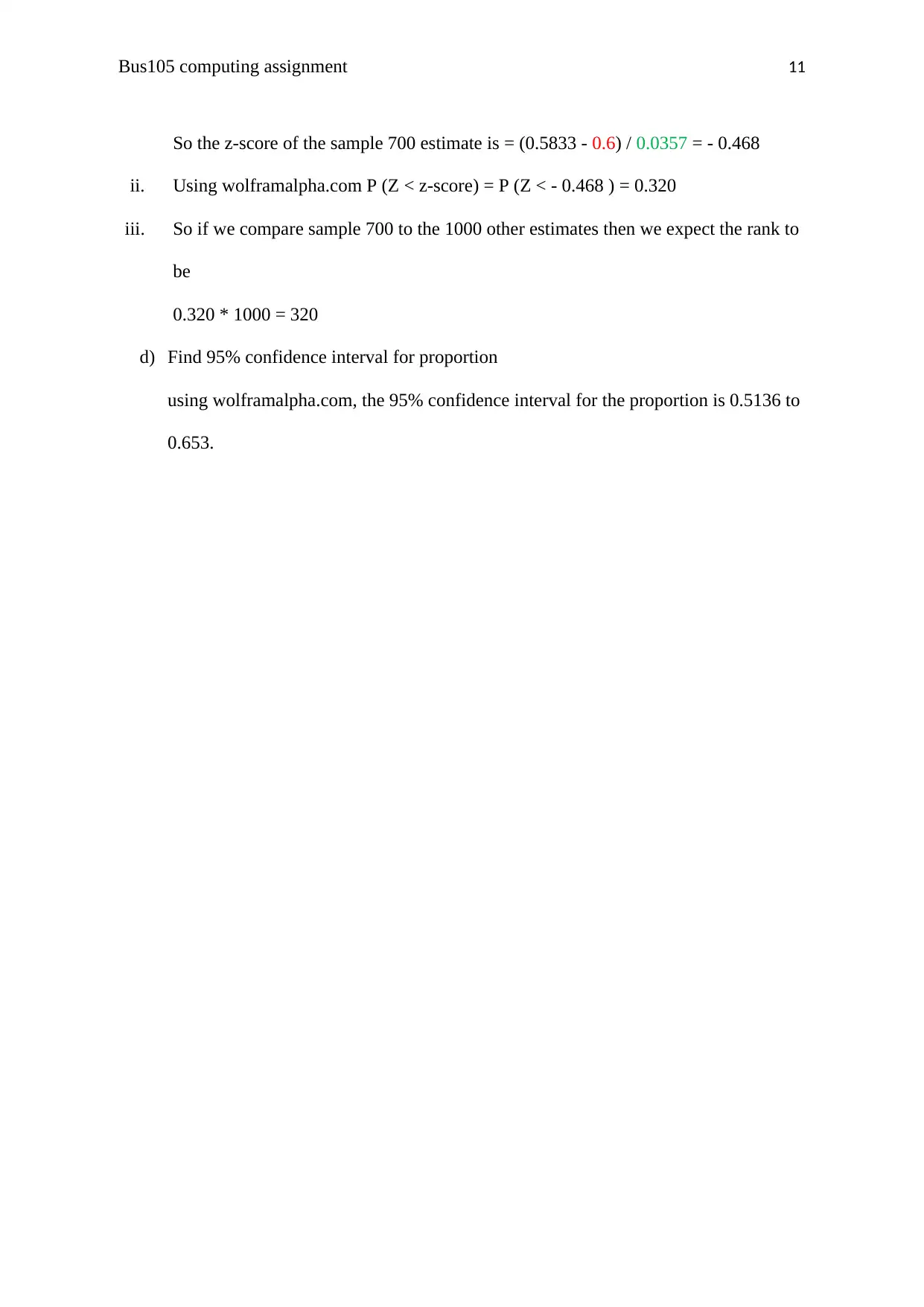
a) Sample 107
Sample 107
Row Labels Count of do you support proposed change?
No 80
Yes 112
Grand Total 192
b) Sample size n is 192 , Sample proportion of people that say yes is ^p = 112 / 192 =
0.5833
c)
i. The average of the 1000 estimates is 0.6 with standard deviation 0.0357
Based on the bars on the right side of the back to back histogram, one can see a curved
pattern. On the left side, a jagged pattern is observed. Thus, it is evident that the terms used
by the students and the administration staff do not quite match in frequency. However, long
bars are at the bottom while the short bars are t the top thereby implying that the
discrepancies are not very big.
*Would a business be able to use back to back histogram?
No. A business would not use a back to back histogram. Though back to back histograms are
visually strong and can compare to normal curves, they cannot read exact values of variables
since the data is grouped into categories. As a result, it will be difficult to compare two data
sets.
Section 6
a) Sample 107
Sample 107
Row Labels Count of do you support proposed change?
No 80
Yes 112
Grand Total 192
b) Sample size n is 192 , Sample proportion of people that say yes is ^p = 112 / 192 =
0.5833
c)
i. The average of the 1000 estimates is 0.6 with standard deviation 0.0357
Secure Best Marks with AI Grader
Need help grading? Try our AI Grader for instant feedback on your assignments.
Bus105 computing assignment 11
So the z-score of the sample 700 estimate is = (0.5833 - 0.6) / 0.0357 = - 0.468
ii. Using wolframalpha.com P (Z < z-score) = P (Z < - 0.468 ) = 0.320
iii. So if we compare sample 700 to the 1000 other estimates then we expect the rank to
be
0.320 * 1000 = 320
d) Find 95% confidence interval for proportion
using wolframalpha.com, the 95% confidence interval for the proportion is 0.5136 to
0.653.

Bus105 computing assignment 12
Reference:
Chen, H., Chiang, R.H. and Storey, V.C., 2012. Business intelligence and analytics: From big
data to big impact. MIS quarterly, 36(4).
Johnson, R.A. and Wichern, D.W., 2014. Applied multivariate statistical analysis (Vol. 4).
New Jersey: Prentice-Hall.
Reference:
Chen, H., Chiang, R.H. and Storey, V.C., 2012. Business intelligence and analytics: From big
data to big impact. MIS quarterly, 36(4).
Johnson, R.A. and Wichern, D.W., 2014. Applied multivariate statistical analysis (Vol. 4).
New Jersey: Prentice-Hall.
Bus105 computing assignment 13
Appendix 1
Figures
Figure 1: Sample 107 scatter plot
10,000 20,000 30,000 40,000 50,000 60,000
$8,000
$10,000
$12,000
$14,000
$16,000
$18,000
$20,000
$22,000
f(x) = − 0.158496496105284 x + 19253.0627207946
Distance travelled
Selling price
Figure 2: Sample 1 proportions
N y
14.10%
85.90%
30.77%
78.95%
Proportions
A B
Figure 3: Simple back to back histogram
Paraphrase This Document
Need a fresh take? Get an instant paraphrase of this document with our AI Paraphraser
Bus105 computing assignment 14
Bus105 computing assignment 15
Tables
Table 1: Sample 107 summary statistics
Which sample? 107
Count of Do they like it? (y=yes, n=no) Column Labels
Row Labels N y
Grand
Total
A 11 67 78
B 24 90 114
Grand Total 35 157 192
Which sample? 107
Count of Do they like it? (y=yes, n=no) Column Labels
Row Labels N y
Grand
Total
A 14.10% 85.90% 100.00%
B 30.77% 78.95% 100.00%
Grand Total 18.23% 81.77% 100.00%
Table 2: Sample 107 summary statistics
Which sample? 107
Values
Row Labels
Count of which machine?
(A or B)
Average of $ Casino
profit from bet
StdDev of $ Casino
profit from bet
A 105 0.142857143 4.539206495
B 95 -0.010526316 1.425413242
Bus105 computing assignment 16
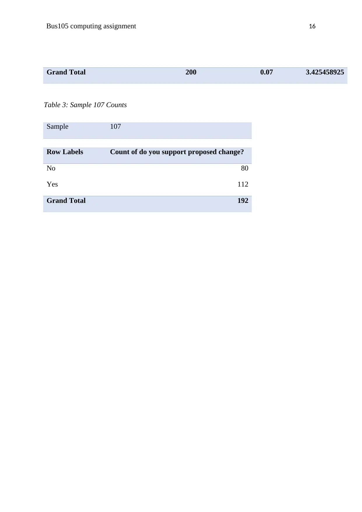
Grand Total 200 0.07 3.425458925
Table 3: Sample 107 Counts
Sample 107
Row Labels Count of do you support proposed change?
No 80
Yes 112
Grand Total 192
Grand Total 200 0.07 3.425458925
Table 3: Sample 107 Counts
Sample 107
Row Labels Count of do you support proposed change?
No 80
Yes 112
Grand Total 192
1 out of 16
Related Documents


Your All-in-One AI-Powered Toolkit for Academic Success.
+13062052269
info@desklib.com
Available 24*7 on WhatsApp / Email
![[object Object]](/_next/static/media/star-bottom.7253800d.svg)
Unlock your academic potential
© 2024 | Zucol Services PVT LTD | All rights reserved.