Multi Regression Analysis and Variable Selection

This assignment focuses on analyzing a multi regression model presented in tables. Students are asked to interpret the coefficients, assess the significance of variables (X2, X4, and X5), and explain how variable selection was used to improve the model by removing insignificant variables (X3 and X6). The analysis should highlight the relationship between independent variables and the dependent variable.

Business analysis 1
Title
Student’s name
Course title
Date

Business analysis 2
TASK 1
Question one
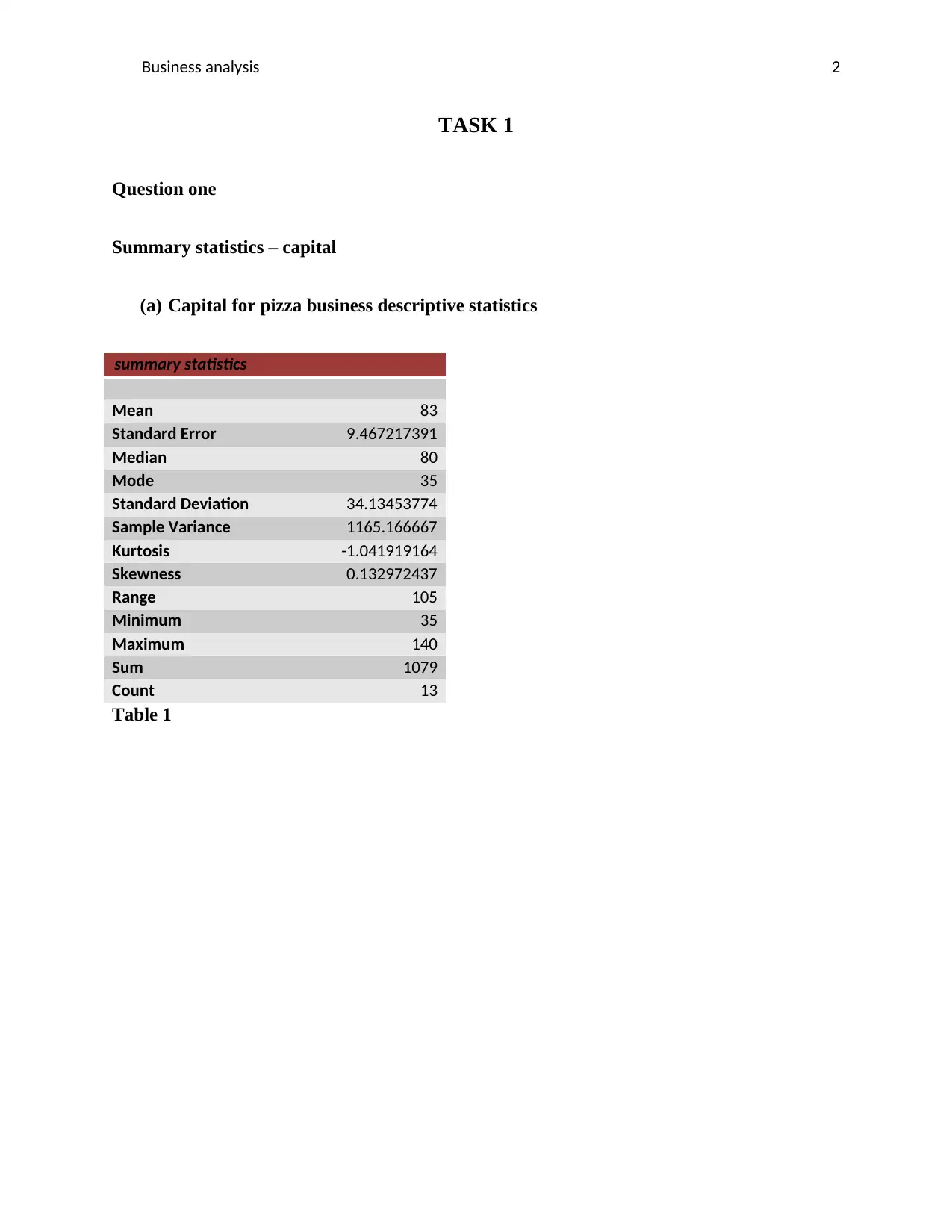
Summary statistics – capital
(a) Capital for pizza business descriptive statistics
summary statistics
Mean 83
Standard Error 9.467217391
Median 80
Mode 35
Standard Deviation 34.13453774
Sample Variance 1165.166667
Kurtosis -1.041919164
Skewness 0.132972437
Range 105
Minimum 35
Maximum 140
Sum 1079
Count 13
Table 1

Business analysis 3
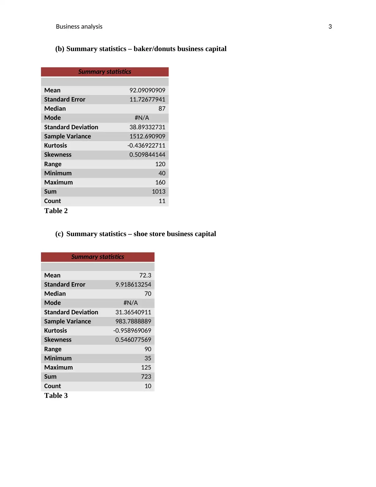
(b) Summary statistics – baker/donuts business capital
Summary statistics
Mean 92.09090909
Standard Error 11.72677941
Median 87
Mode #N/A
Standard Deviation 38.89332731
Sample Variance 1512.690909
Kurtosis -0.436922711
Skewness 0.509844144
Range 120
Minimum 40
Maximum 160
Sum 1013
Count 11
Table 2
(c) Summary statistics – shoe store business capital
Summary statistics
Mean 72.3
Standard Error 9.918613254
Median 70
Mode #N/A
Standard Deviation 31.36540911
Sample Variance 983.7888889
Kurtosis -0.958969069
Skewness 0.546077569
Range 90
Minimum 35
Maximum 125
Sum 723
Count 10
Table 3

Business analysis 4
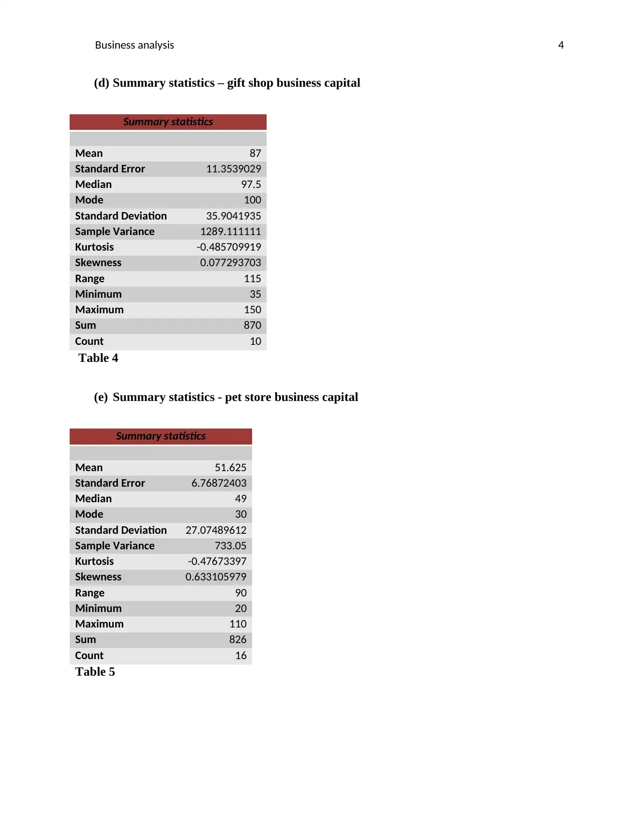
(d) Summary statistics – gift shop business capital
Summary statistics
Mean 87
Standard Error 11.3539029
Median 97.5
Mode 100
Standard Deviation 35.9041935
Sample Variance 1289.111111
Kurtosis -0.485709919
Skewness 0.077293703
Range 115
Minimum 35
Maximum 150
Sum 870
Count 10
Table 4
(e) Summary statistics - pet store business capital
Summary statistics
Mean 51.625
Standard Error 6.76872403
Median 49
Mode 30
Standard Deviation 27.07489612
Sample Variance 733.05
Kurtosis -0.47673397
Skewness 0.633105979
Range 90
Minimum 20
Maximum 110
Sum 826
Count 16
Table 5

Business analysis 5
Question 2
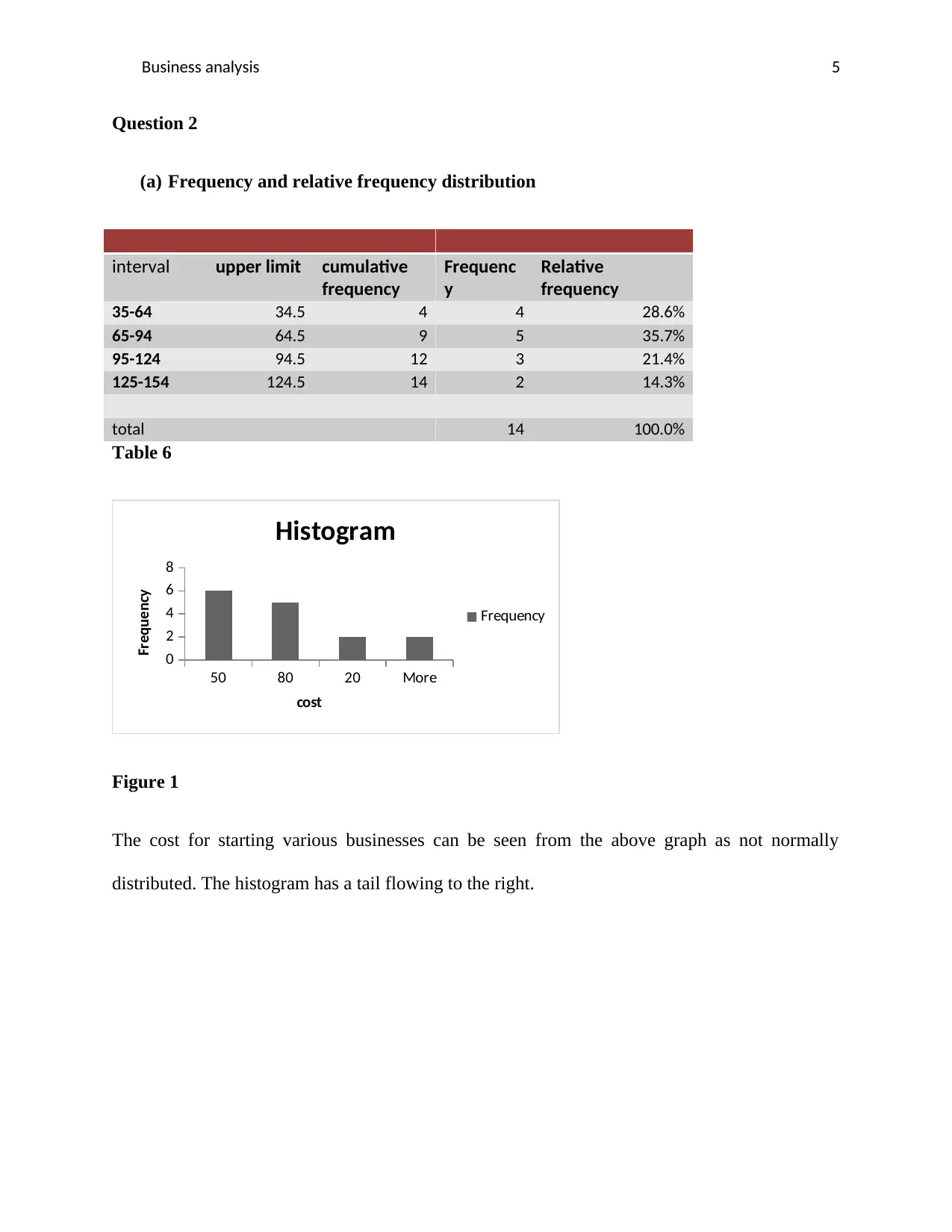
(a) Frequency and relative frequency distribution
interval upper limit cumulative
frequency
Frequenc
y
Relative
frequency
35-64 34.5 4 4 28.6%
65-94 64.5 9 5 35.7%
95-124 94.5 12 3 21.4%
125-154 124.5 14 2 14.3%
total 14 100.0%
Table 6
50 80 20 More
0
2
4
6
8
Histogram
Frequency
cost
Frequency
Figure 1
The cost for starting various businesses can be seen from the above graph as not normally
distributed. The histogram has a tail flowing to the right.

Business analysis 6
Question 3
X1 X2 X3 X4 X5
Mean 83 Mean 92.090
9
Mean 72.3 Mean 87 Mean 51.625
Media
n
80 Media
n
87 Media
n
70 Media
n
97.5 Media
n
49
Mode 35 Mode #N/A Mode #N/A Mode 100 Mode 30
Std
Dev.
34.13
5
Std
Dev.
38.893
3
Std
Dev.
31.36
5
Std
Dev.
35.90
4
Std
Dev.
27.074
9
Var 1165.
2
Var 1512.6
9
Var 983.7
9
Var 1289.
1
Var 733.05
Range 105 Range 120 Range 90 Range 115 Range 90
Count 13 Count 11 Count 10 Count 10 Count 16
Table 7
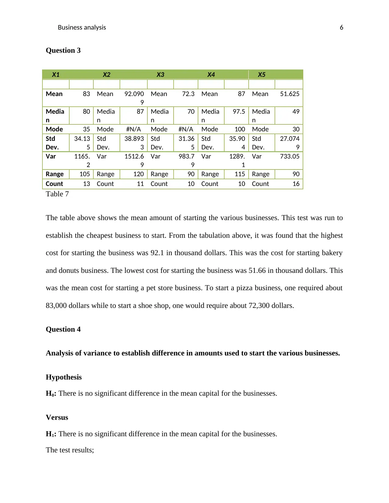
The table above shows the mean amount of starting the various businesses. This test was run to
establish the cheapest business to start. From the tabulation above, it was found that the highest
cost for starting the business was 92.1 in thousand dollars. This was the cost for starting bakery
and donuts business. The lowest cost for starting the business was 51.66 in thousand dollars. This
was the mean cost for starting a pet store business. To start a pizza business, one required about
83,000 dollars while to start a shoe shop, one would require about 72,300 dollars.
Question 4
Analysis of variance to establish difference in amounts used to start the various businesses.
Hypothesis
H0: There is no significant difference in the mean capital for the businesses.
Versus
H1: There is no significant difference in the mean capital for the businesses.
The test results;

Business analysis 7
SUMMARY
Groups Count Sum Average Varianc
e
X1 13 1079 83 1165.16
7
X2 11 1013 92.0909
1
1512.69
1
X3 10 723 72.3 983.788
9
X4 10 870 87 1289.11
1
X5 16 826 51.625 733.05
ANOVA
Source of
Variation
SS df MS F P-value F crit
Between Groups 14298.2
2
4 3574.55
6
3.24633
6
0.01839
1
2.53968
9
Within Groups 60560.7
6
55 1101.10
5
Total 74858.9
8
59
Table 8
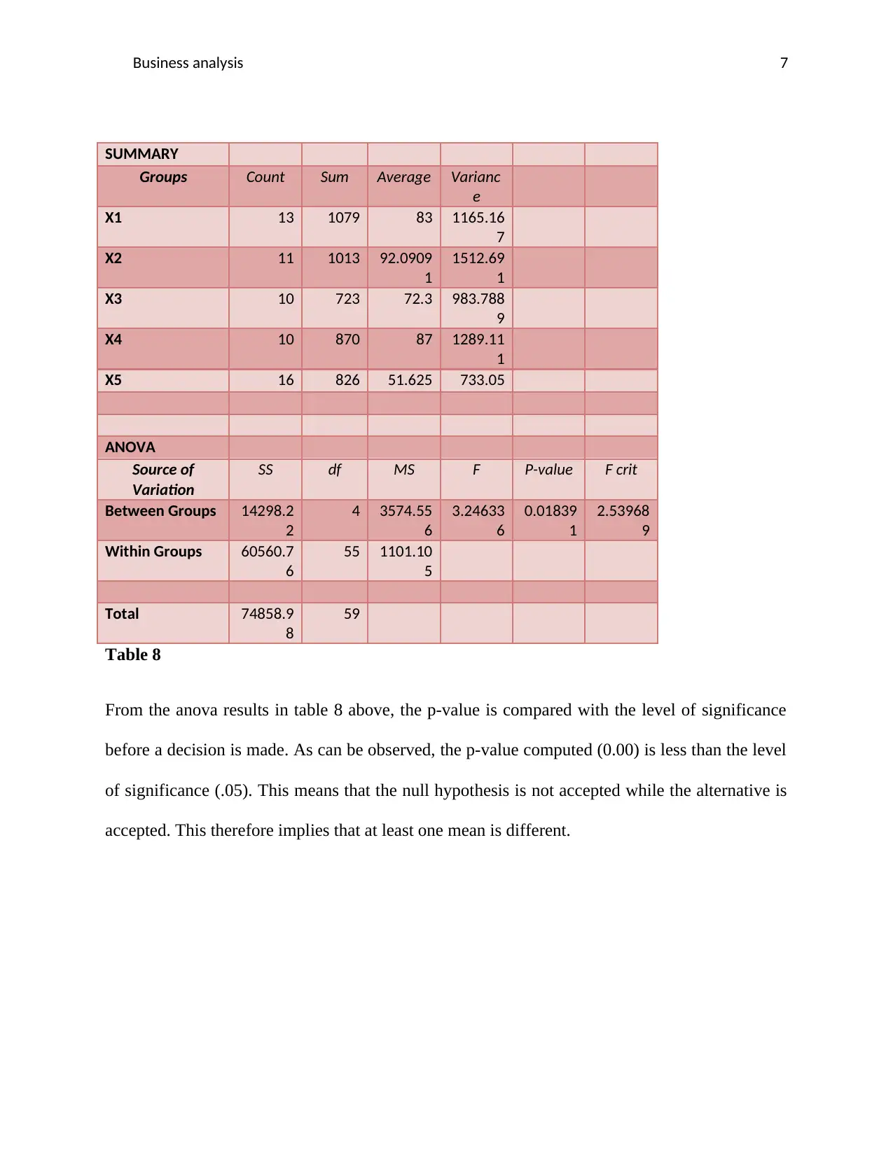
From the anova results in table 8 above, the p-value is compared with the level of significance
before a decision is made. As can be observed, the p-value computed (0.00) is less than the level
of significance (.05). This means that the null hypothesis is not accepted while the alternative is
accepted. This therefore implies that at least one mean is different.

Business analysis 8
TASK 2
Question 1
SUMMARY OUTPUT
Regression Statistics
Multiple R 0.996584
R Square 0.993179
Adjusted R
Square
0.991556
Standard
Error
17.64924
Observation
s
27
ANOVA
df SS MS F Significan
ce F
Regression 5 952538.9 19050 611.590 5.4E-22
Residual 21 6541.41 311.49
Total 26 959080.4
Coefficien
ts
Standard
Error
t Stat P-value Lower
95%
Upper
95%
Lower
95.0%
Upper
95.0%
Intercept -18.8594 30.15023 -
0.6255
1
0.53837
2
-81.5602 43.8414
2
-
81.5602
43.8414
2
X Variable 2 16.20157 3.544437 4.5709 0.00016 8.830513 23.5726 8.83051 23.5726
X Variable 3 0.174635 0.057606 3.0315 0.00634 0.054837 0.29443 0.05483 0.29443
X Variable 4 11.52627 2.532103 4.5520 0.00017 6.260472 16.7920 6.26047 16.7920
X Variable 5 13.58031 1.770457 7.6705 1.61E-0 9.898447 17.2621 9.89844 17.2621
X Variable 6 -5.31097 1.705427 -
3.1141
0.00524 -8.8576 -
1.76434
-8.8576 -
1.76434

Business analysis 9
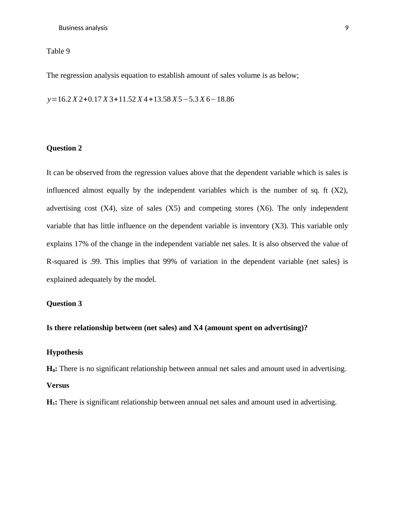
Table 9
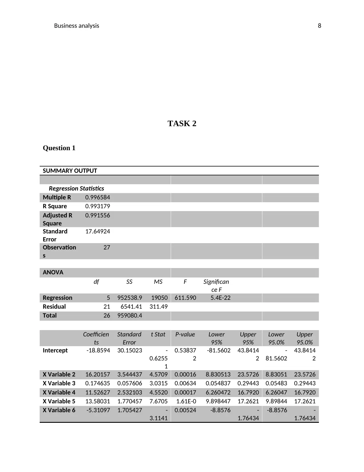
The regression analysis equation to establish amount of sales volume is as below;
y=16.2 X 2+0.17 X 3+11.52 X 4 +13.58 X 5−5.3 X 6−18.86
Question 2
It can be observed from the regression values above that the dependent variable which is sales is
influenced almost equally by the independent variables which is the number of sq. ft (X2),
advertising cost (X4), size of sales (X5) and competing stores (X6). The only independent
variable that has little influence on the dependent variable is inventory (X3). This variable only
explains 17% of the change in the independent variable net sales. It is also observed the value of
R-squared is .99. This implies that 99% of variation in the dependent variable (net sales) is
explained adequately by the model.
Question 3
Is there relationship between (net sales) and X4 (amount spent on advertising)?
Hypothesis
H0: There is no significant relationship between annual net sales and amount used in advertising.
Versus
H1: There is significant relationship between annual net sales and amount used in advertising.

Business analysis 10
t-Test: Paired Two Sample for Means
annual net
sales
advertising
cost
Mean 286.5740741 8.099999982
Variance 36887.70584 14.24692313
Observations 27 27
Pearson Correlation 0.914024075
Hypothesized Mean Difference 0
df 26
t Stat 7.671559165
P(T<=t) one-tail 1.92341E-08
t Critical one-tail 1.70561792
P(T<=t) two-tail 3.84681E-08
t Critical two-tail 2.055529439
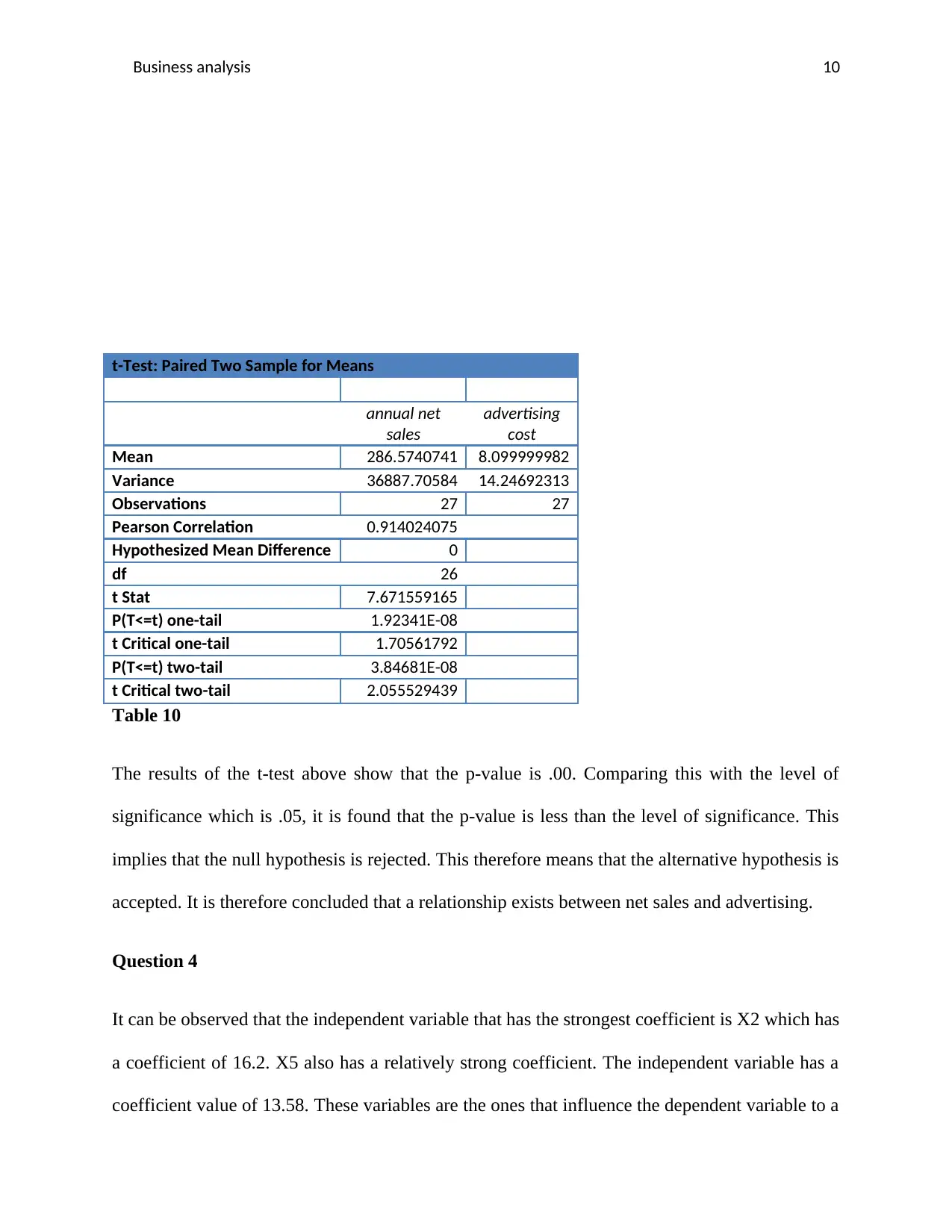
Table 10
The results of the t-test above show that the p-value is .00. Comparing this with the level of
significance which is .05, it is found that the p-value is less than the level of significance. This
implies that the null hypothesis is rejected. This therefore means that the alternative hypothesis is
accepted. It is therefore concluded that a relationship exists between net sales and advertising.
Question 4
It can be observed that the independent variable that has the strongest coefficient is X2 which has
a coefficient of 16.2. X5 also has a relatively strong coefficient. The independent variable has a
coefficient value of 13.58. These variables are the ones that influence the dependent variable to a

Business analysis 11
larger extent. The variable with the least coefficient is X6. It has a coefficient value of 5.3. It
causes the least variation on the dependent variable with a unit change in it.
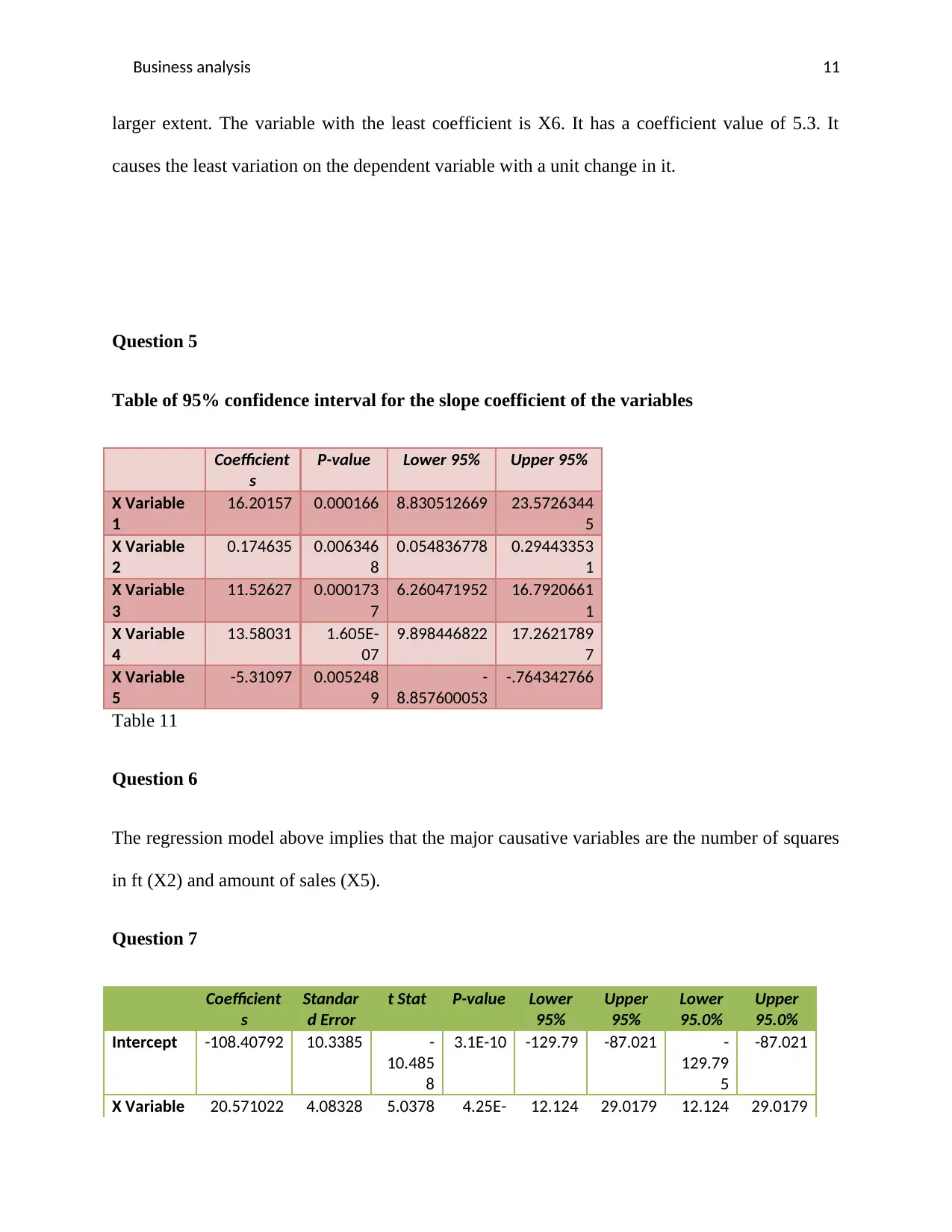
Question 5
Table of 95% confidence interval for the slope coefficient of the variables
Coefficient
s
P-value Lower 95% Upper 95%
X Variable
1
16.20157 0.000166 8.830512669 23.5726344
5
X Variable
2
0.174635 0.006346
8
0.054836778 0.29443353
1
X Variable
3
11.52627 0.000173
7
6.260471952 16.7920661
1
X Variable
4
13.58031 1.605E-
07
9.898446822 17.2621789
7
X Variable
5
-5.31097 0.005248
9
-
8.857600053
-.764342766
Table 11
Question 6
The regression model above implies that the major causative variables are the number of squares
in ft (X2) and amount of sales (X5).
Question 7
Coefficient
s
Standar
d Error
t Stat P-value Lower
95%
Upper
95%
Lower
95.0%
Upper
95.0%
Intercept -108.40792 10.3385 -
10.485
8
3.1E-10 -129.79 -87.021 -
129.79
5
-87.021
X Variable 20.571022 4.08328 5.0378 4.25E- 12.124 29.0179 12.124 29.0179

Business analysis 12
2 6 1
X Variable
4
19.086839 1.95871 9.7445
6
1.24E- 15.034 23.1387 15.034
9
23.1387
X Variable
5
17.741477 1.74783 10.150
5
5.76E-1 14.125
8
21.3571
6
14.125
8
21.3571
6
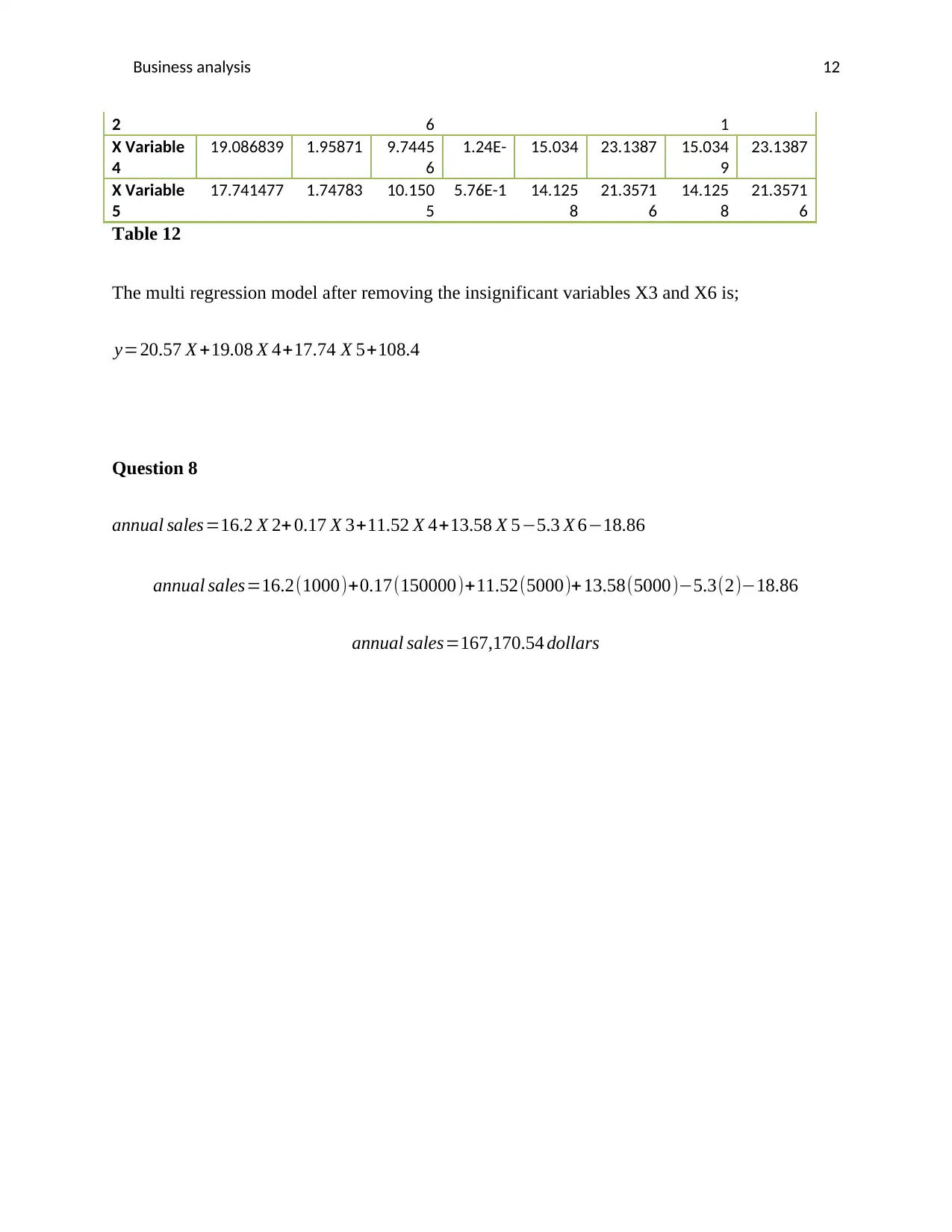
Table 12
The multi regression model after removing the insignificant variables X3 and X6 is;
y=20.57 X +19.08 X 4+17.74 X 5+108.4
Question 8
annual sales=16.2 X 2+ 0.17 X 3+11.52 X 4+13.58 X 5−5.3 X 6−18.86
annual sales=16.2(1000)+0.17(150000)+11.52(5000)+ 13.58(5000)−5.3(2)−18.86
annual sales=167,170.54 dollars