Business Analytics and Statistics Assignment - Sunshine Coast

Running head: BUSINESS ANALYTICS AND STATISTICS
Business analytics and Statistics
Name:
Institution:

BUSINESS ANALYTICS AND STATISTICS
Table of Contents
Table of Contents.......................................................................................................................2
Introduction................................................................................................................................3
Results and discussion................................................................................................................3
Business performance............................................................................................................3
Business performance by product location in the shop..........................................................4
Business payment performance..............................................................................................7
Average sales by the month of the year.................................................................................9
Net sales by the season of the year.......................................................................................10
Gross profit by month of the year........................................................................................11
Association between net sales and month of the year..........................................................13
Regression model.................................................................................................................14
Conclusion................................................................................................................................14
References................................................................................................................................16

BUSINESS ANALYTICS AND STATISTICS
Introduction
This report will use longitudinal and cross-sectional data collected from a small health food
shop on the Sunshine Coast. The main area of emphasized is the sales and profit yield. It is
thought that there is a profit difference by the area of sale, the season of the year and month
of the year. Therefore, the data will help determine whether the profit, and net sale made
during different times of the year, and places significantly differ. Among other objectives, the
research pointed out business performance, which can help make business decisions. Among
others, the research computed descriptive statistics for the shop to give an overview of the
business performance. Second, several statistical tests were carried out to determine which
product is the best performing; which location is returning the highest revenue/sales, whether
profit by month/season significantly differs. The data were refined, where the data
measurement scales for Location of product in the shop, Product Class (number), Product
Class and Product Name were changed from the ordinal scale to nominal scale. Similar
changes were made for the Season of the year, Month of the year, and Weekday.
Results and discussion
Business performance
a. The total sales by the product class
The summary of the descriptive statistics of the total sales by the product class. It indicates
that the water has the highest average sales of $1,866.88 (SD = $2,541.63). The second best
performing product class is fruit (M= $1,048.68, SD = $2,469.41). The product class that is
not performing well (worst performing) is juicing with an average sale of $5.00, and second
worse performing product class is $17.96 (SD = $24.37).
b. The total profit by the product class
The summary of the descriptive statistics is as follows.

BUSINESS ANALYTICS AND STATISTICS
The product class with the highest average profit is water (M = $884.25, SD = $1,188.12),
and second-best performing is fruit (M = $530.73, SD = $1,247.33). The worse performing
product is the Juicing ($3.00).
Business performance by product location in the shop
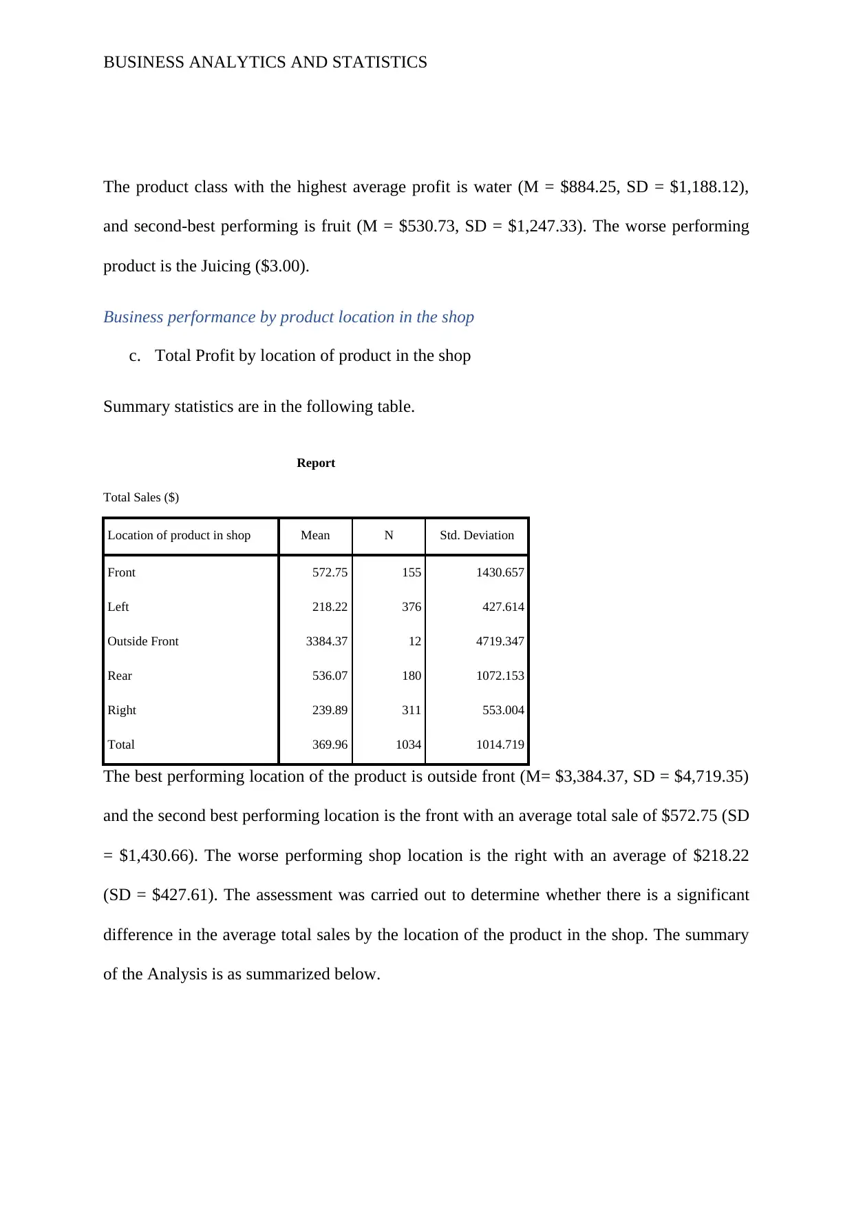
c. Total Profit by location of product in the shop
Summary statistics are in the following table.
Report
Total Sales ($)
Location of product in shop Mean N Std. Deviation
Front 572.75 155 1430.657
Left 218.22 376 427.614
Outside Front 3384.37 12 4719.347
Rear 536.07 180 1072.153
Right 239.89 311 553.004
Total 369.96 1034 1014.719
The best performing location of the product is outside front (M= $3,384.37, SD = $4,719.35)
and the second best performing location is the front with an average total sale of $572.75 (SD
= $1,430.66). The worse performing shop location is the right with an average of $218.22
(SD = $427.61). The assessment was carried out to determine whether there is a significant
difference in the average total sales by the location of the product in the shop. The summary
of the Analysis is as summarized below.

BUSINESS ANALYTICS AND STATISTICS
ANOVA Table
Sum of Squares df Mean Square F Sig.
Total Sales ($) * Location
of product in shop
Between Groups (Combined) 134299725.024 4 33574931.256 37.176 .000
Within Groups 929333380.817 1029 903142.255
Total 1063633105.841 1033
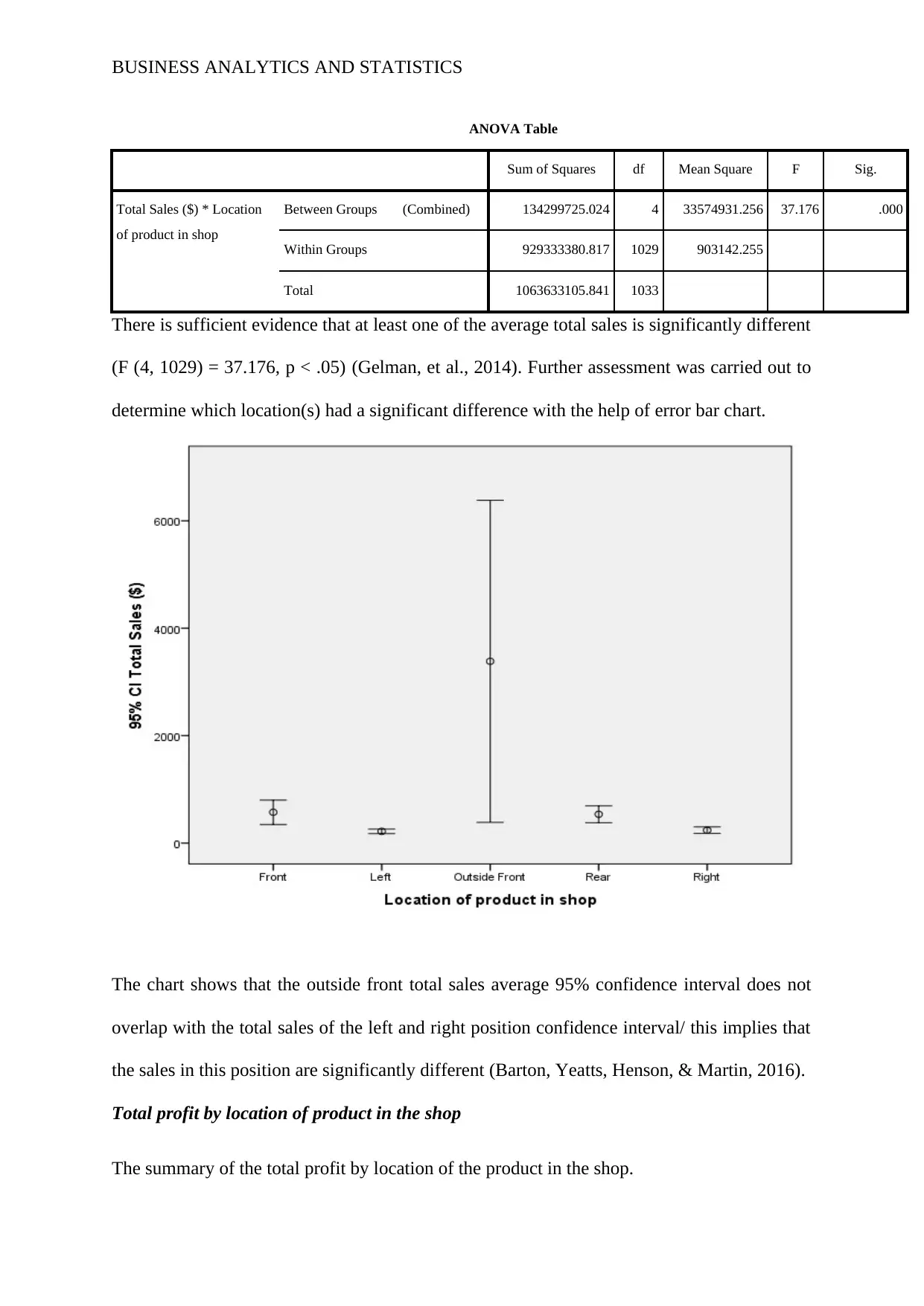
There is sufficient evidence that at least one of the average total sales is significantly different
(F (4, 1029) = 37.176, p < .05) (Gelman, et al., 2014). Further assessment was carried out to
determine which location(s) had a significant difference with the help of error bar chart.
The chart shows that the outside front total sales average 95% confidence interval does not
overlap with the total sales of the left and right position confidence interval/ this implies that
the sales in this position are significantly different (Barton, Yeatts, Henson, & Martin, 2016).
Total profit by location of product in the shop
The summary of the total profit by location of the product in the shop.

BUSINESS ANALYTICS AND STATISTICS
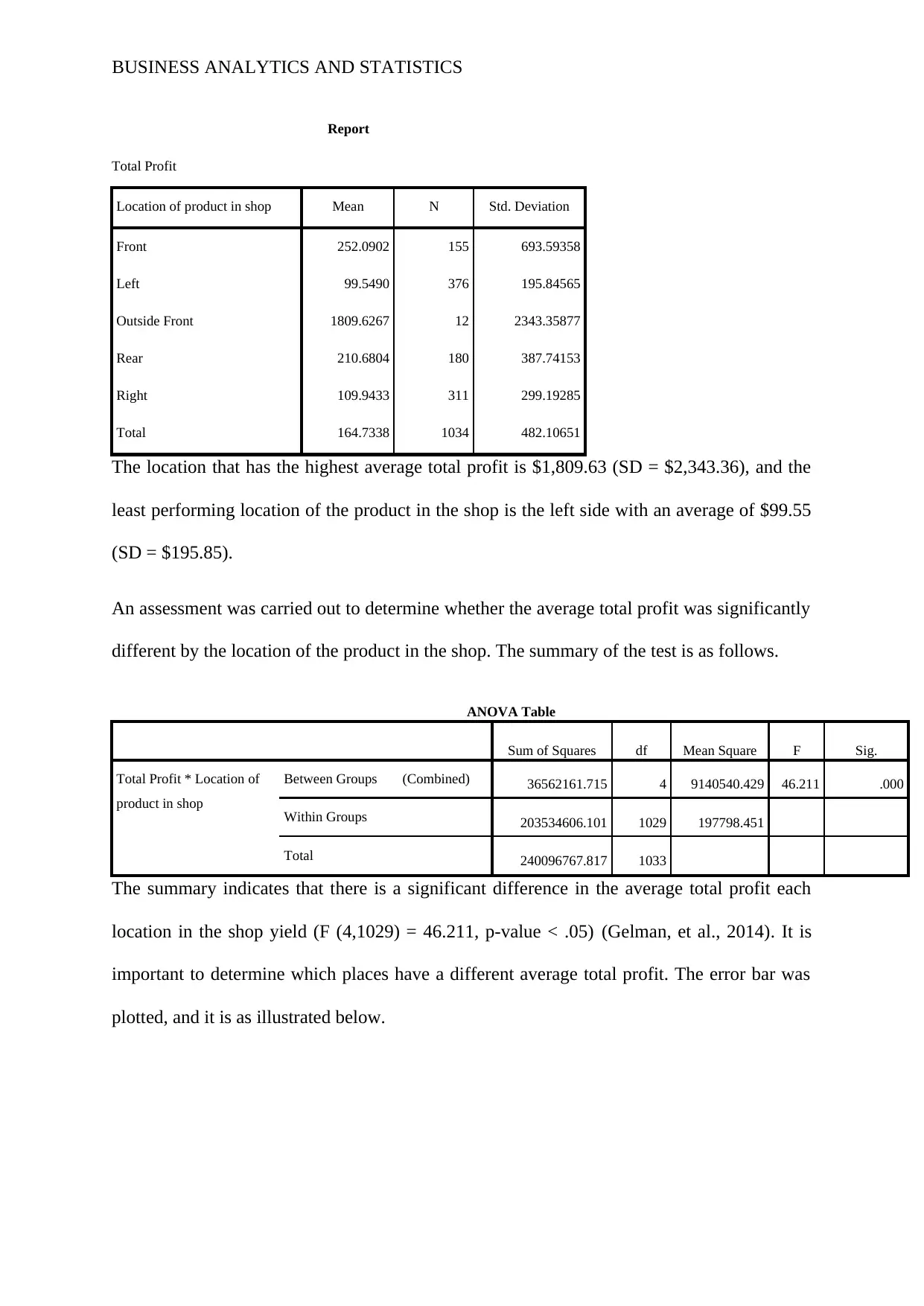
Report
Total Profit
Location of product in shop Mean N Std. Deviation
Front 252.0902 155 693.59358
Left 99.5490 376 195.84565
Outside Front 1809.6267 12 2343.35877
Rear 210.6804 180 387.74153
Right 109.9433 311 299.19285
Total 164.7338 1034 482.10651
The location that has the highest average total profit is $1,809.63 (SD = $2,343.36), and the
least performing location of the product in the shop is the left side with an average of $99.55
(SD = $195.85).
An assessment was carried out to determine whether the average total profit was significantly
different by the location of the product in the shop. The summary of the test is as follows.
ANOVA Table
Sum of Squares df Mean Square F Sig.
Total Profit * Location of
product in shop
Between Groups (Combined) 36562161.715 4 9140540.429 46.211 .000
Within Groups 203534606.101 1029 197798.451
Total 240096767.817 1033
The summary indicates that there is a significant difference in the average total profit each
location in the shop yield (F (4,1029) = 46.211, p-value < .05) (Gelman, et al., 2014). It is
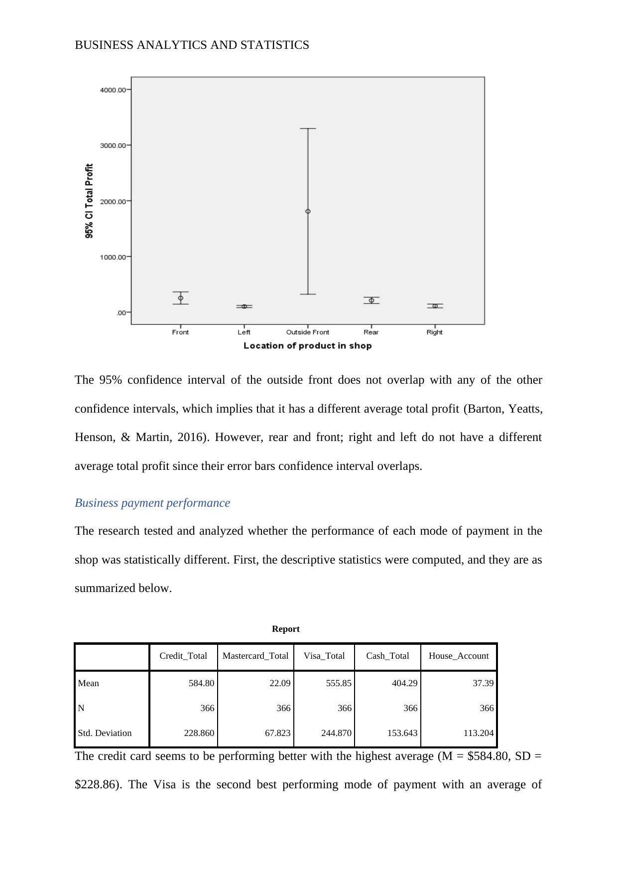
important to determine which places have a different average total profit. The error bar was
plotted, and it is as illustrated below.

BUSINESS ANALYTICS AND STATISTICS
The 95% confidence interval of the outside front does not overlap with any of the other
confidence intervals, which implies that it has a different average total profit (Barton, Yeatts,
Henson, & Martin, 2016). However, rear and front; right and left do not have a different
average total profit since their error bars confidence interval overlaps.
Business payment performance
The research tested and analyzed whether the performance of each mode of payment in the
shop was statistically different. First, the descriptive statistics were computed, and they are as
summarized below.
Report
Credit_Total Mastercard_Total Visa_Total Cash_Total House_Account
Mean 584.80 22.09 555.85 404.29 37.39
N 366 366 366 366 366
Std. Deviation 228.860 67.823 244.870 153.643 113.204
The credit card seems to be performing better with the highest average (M = $584.80, SD =
$228.86). The Visa is the second best performing mode of payment with an average of

BUSINESS ANALYTICS AND STATISTICS
$555.85 (SD = $244.87). The method that seems to be performing poorly is the Mastercard
with the lowest average of $22.09 (SD = $67.82). However, although there seem to a
difference in the average, it is imperative to test the hypothesis. Therefore, the hypothesis at
the level .05, whether the methods of payment were performing differently.
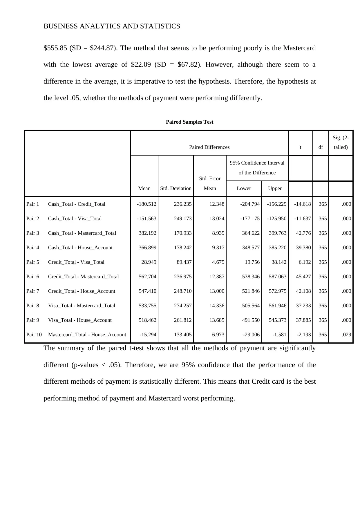
Paired Samples Test
Paired Differences t df
Sig. (2-
tailed)
Mean Std. Deviation
Std. Error
Mean
95% Confidence Interval
of the Difference
Lower Upper
Pair 1 Cash_Total - Credit_Total -180.512 236.235 12.348 -204.794 -156.229 -14.618 365 .000
Pair 2 Cash_Total - Visa_Total -151.563 249.173 13.024 -177.175 -125.950 -11.637 365 .000
Pair 3 Cash_Total - Mastercard_Total 382.192 170.933 8.935 364.622 399.763 42.776 365 .000
Pair 4 Cash_Total - House_Account 366.899 178.242 9.317 348.577 385.220 39.380 365 .000
Pair 5 Credit_Total - Visa_Total 28.949 89.437 4.675 19.756 38.142 6.192 365 .000
Pair 6 Credit_Total - Mastercard_Total 562.704 236.975 12.387 538.346 587.063 45.427 365 .000
Pair 7 Credit_Total - House_Account 547.410 248.710 13.000 521.846 572.975 42.108 365 .000
Pair 8 Visa_Total - Mastercard_Total 533.755 274.257 14.336 505.564 561.946 37.233 365 .000
Pair 9 Visa_Total - House_Account 518.462 261.812 13.685 491.550 545.373 37.885 365 .000
Pair 10 Mastercard_Total - House_Account -15.294 133.405 6.973 -29.006 -1.581 -2.193 365 .029
The summary of the paired t-test shows that all the methods of payment are significantly
different (p-values < .05). Therefore, we are 95% confidence that the performance of the
different methods of payment is statistically different. This means that Credit card is the best
performing method of payment and Mastercard worst performing.

BUSINESS ANALYTICS AND STATISTICS
Average sales by the month of the year
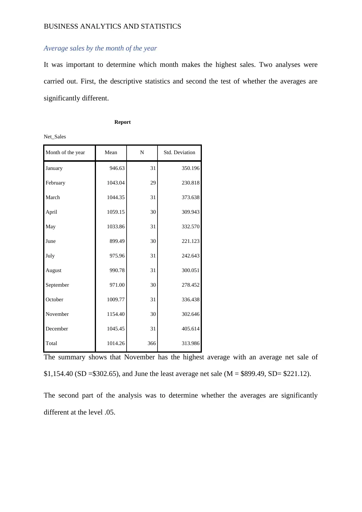
It was important to determine which month makes the highest sales. Two analyses were
carried out. First, the descriptive statistics and second the test of whether the averages are
significantly different.
Report
Net_Sales
Month of the year Mean N Std. Deviation
January 946.63 31 350.196
February 1043.04 29 230.818
March 1044.35 31 373.638
April 1059.15 30 309.943
May 1033.86 31 332.570
June 899.49 30 221.123
July 975.96 31 242.643
August 990.78 31 300.051
September 971.00 30 278.452
October 1009.77 31 336.438
November 1154.40 30 302.646
December 1045.45 31 405.614
Total 1014.26 366 313.986
The summary shows that November has the highest average with an average net sale of
$1,154.40 (SD =$302.65), and June the least average net sale (M = $899.49, SD= $221.12).
The second part of the analysis was to determine whether the averages are significantly
different at the level .05.

BUSINESS ANALYTICS AND STATISTICS
ANOVA Table
Sum of Squares df Mean Square F Sig.
Net_Sales * Month of the
year
Between Groups (Combined) 1399993.227 11 127272.112 1.303 .221
Within Groups 34584296.355 354 97695.752
Total 35984289.582 365
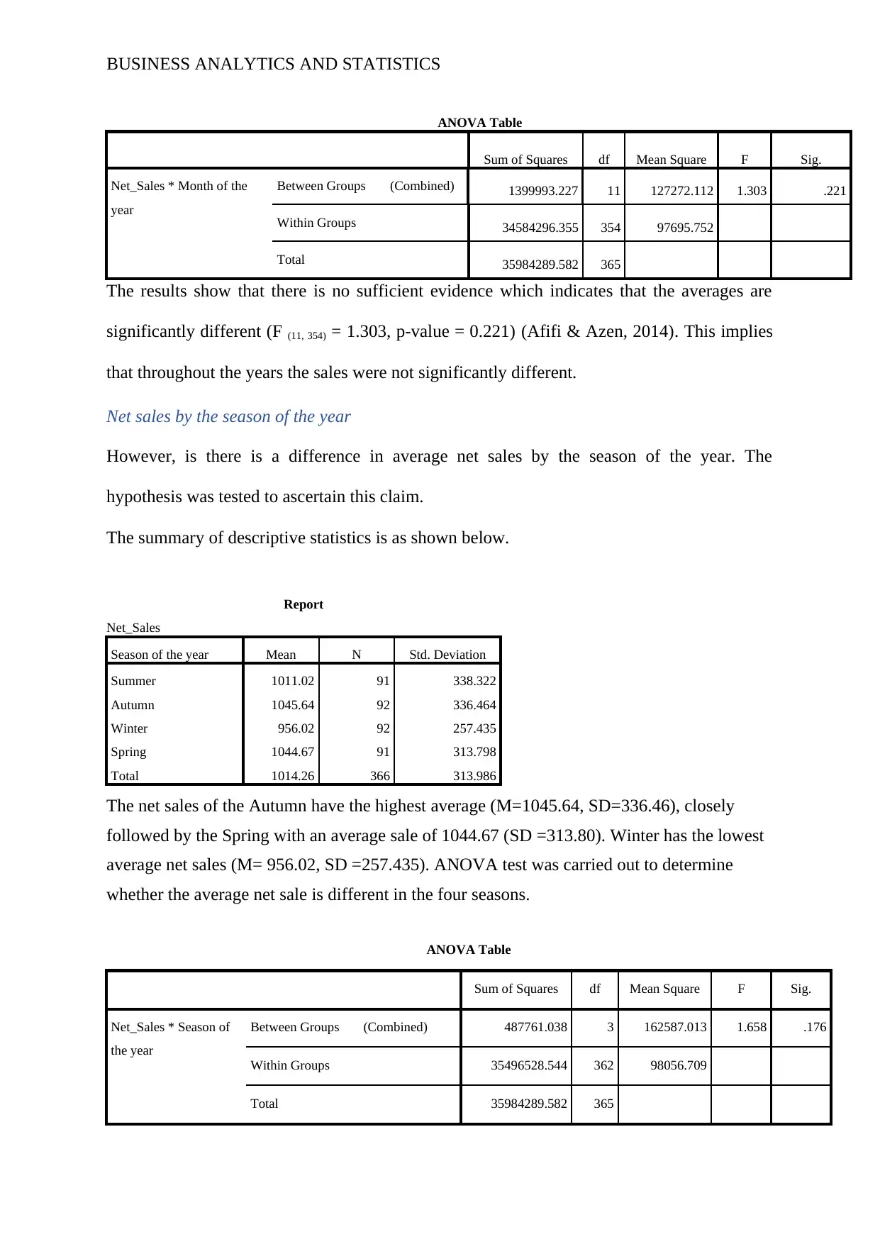
The results show that there is no sufficient evidence which indicates that the averages are
significantly different (F (11, 354) = 1.303, p-value = 0.221) (Afifi & Azen, 2014). This implies
that throughout the years the sales were not significantly different.
Net sales by the season of the year
However, is there is a difference in average net sales by the season of the year. The
hypothesis was tested to ascertain this claim.
The summary of descriptive statistics is as shown below.
Report
Net_Sales
Season of the year Mean N Std. Deviation
Summer 1011.02 91 338.322
Autumn 1045.64 92 336.464
Winter 956.02 92 257.435
Spring 1044.67 91 313.798
Total 1014.26 366 313.986
The net sales of the Autumn have the highest average (M=1045.64, SD=336.46), closely
followed by the Spring with an average sale of 1044.67 (SD =313.80). Winter has the lowest
average net sales (M= 956.02, SD =257.435). ANOVA test was carried out to determine
whether the average net sale is different in the four seasons.
ANOVA Table
Sum of Squares df Mean Square F Sig.
Net_Sales * Season of
the year
Between Groups (Combined) 487761.038 3 162587.013 1.658 .176
Within Groups 35496528.544 362 98056.709
Total 35984289.582 365

BUSINESS ANALYTICS AND STATISTICS
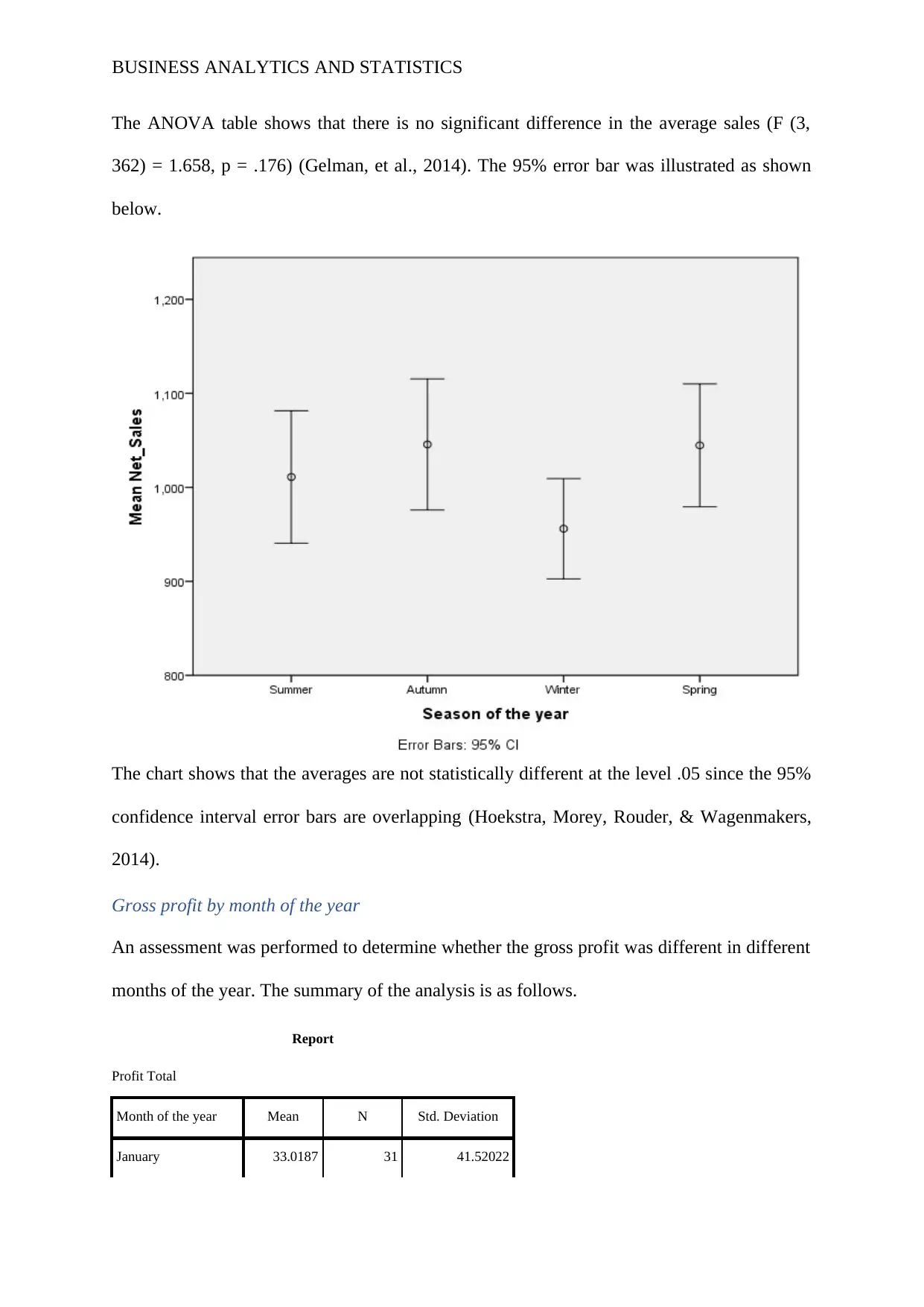
The ANOVA table shows that there is no significant difference in the average sales (F (3,
362) = 1.658, p = .176) (Gelman, et al., 2014). The 95% error bar was illustrated as shown
below.
The chart shows that the averages are not statistically different at the level .05 since the 95%
confidence interval error bars are overlapping (Hoekstra, Morey, Rouder, & Wagenmakers,
2014).
Gross profit by month of the year
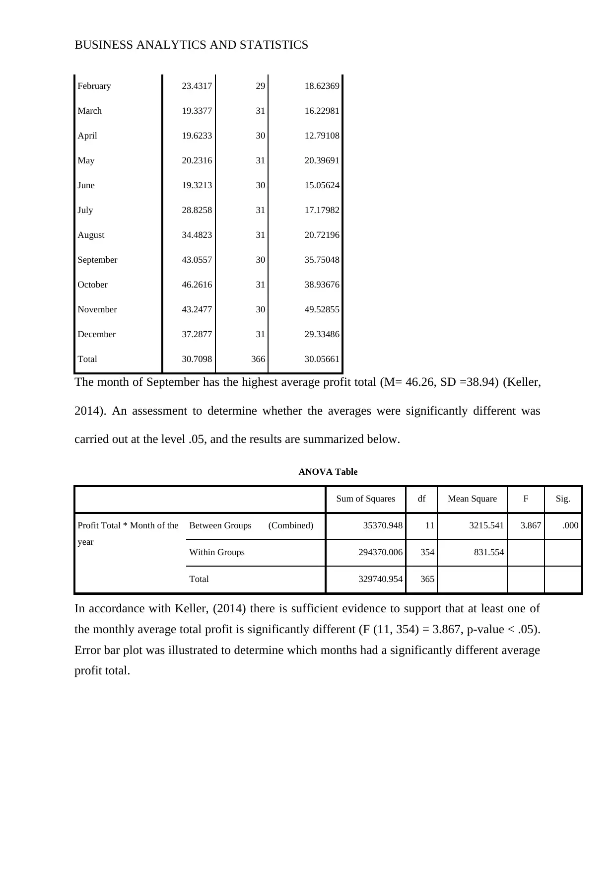
An assessment was performed to determine whether the gross profit was different in different
months of the year. The summary of the analysis is as follows.
Report
Profit Total
Month of the year Mean N Std. Deviation
January 33.0187 31 41.52022

BUSINESS ANALYTICS AND STATISTICS
February 23.4317 29 18.62369
March 19.3377 31 16.22981
April 19.6233 30 12.79108
May 20.2316 31 20.39691
June 19.3213 30 15.05624
July 28.8258 31 17.17982
August 34.4823 31 20.72196
September 43.0557 30 35.75048
October 46.2616 31 38.93676
November 43.2477 30 49.52855
December 37.2877 31 29.33486
Total 30.7098 366 30.05661
The month of September has the highest average profit total (M= 46.26, SD =38.94) (Keller,
2014). An assessment to determine whether the averages were significantly different was
carried out at the level .05, and the results are summarized below.
ANOVA Table
Sum of Squares df Mean Square F Sig.
Profit Total * Month of the
year
Between Groups (Combined) 35370.948 11 3215.541 3.867 .000
Within Groups 294370.006 354 831.554
Total 329740.954 365
In accordance with Keller, (2014) there is sufficient evidence to support that at least one of
the monthly average total profit is significantly different (F (11, 354) = 3.867, p-value < .05).
Error bar plot was illustrated to determine which months had a significantly different average
profit total.

BUSINESS ANALYTICS AND STATISTICS
The 95% confidence interval indicates that some of the months like March-June are
significantly different from the averages of September and August. This is because, their
intervals do not overlap (Afifi & Azen, 2014).
Association between net sales and month of the year
Notably, the net sales are on an interval scale and the month of the year in nominal scale,
hence the most appropriate method of assessing whether there is an association is using Eta.
This was carried out, and the results are as follows.
Directional Measures
Value
Nominal by Interval Eta Net_Sales Dependent .197
Month of the year Dependent .982

BUSINESS ANALYTICS AND STATISTICS
The Eta value is 0.197, and as a general rule, this shows that there is a small effect of month
of the year on net sale (Keller, 2014). This effect is not significant.
Regression model
A model was developed to determine whether there is a significant association between net
sales and the rainfall amount. The net sales were considered as the dependent variable and the
rainfall as the factor variable.
Model Summaryb
Model R R Square
Adjusted R
Square
Std. Error of the
Estimate Durbin-Watson
1 .035a .001 -.002 314.624 2.140
a. Predictors: (Constant), Rainfall
b. Dependent Variable: Net_Sales
ANOVAa
Model Sum of Squares df Mean Square F Sig.
1 Regression 44891.857 1 44891.857 .454 .501b
Residual 35932762.123 363 98988.325
Total 35977653.981 364
a. Dependent Variable: Net_Sales
b. Predictors: (Constant), Rainfall
The coefficient of determination shows that only 0.1% of the variation of net sales can be
explained by the rainfall. Further, the Durbin-Watson value is 2.140 which shows that there is
no correlation between the residuals (Keller, 2014). The regression model is not significant (F
(1, 363) =0.454, p-value = 0.501). Thus, we can conclude that rainfall is not associated with
net sales.
Conclusion
The findings of the research are as follows:

BUSINESS ANALYTICS AND STATISTICS
 The total profit by the location of the product in the shop is significantly different.
This means that different location in the shop has a different return.
 Total profit yield at different location of the product in the shop is significantly
different.
 The average of different methods of payment is different.
 The average net sales all months throughout the year were not different.
 At least one of the monthly average total profit is significantly different.
 There is a small effect of month on net sale.
 Rainfall is not associated with net sales.

BUSINESS ANALYTICS AND STATISTICS
References
Afifi, A. A., & Azen, S. P. (2014). Statistical analysis: a computer oriented approach.
Academic press.
Barton, M., Yeatts, P. E., Henson, R. K., & Martin, S. B. (2016). Moving beyond univariate
post-hoc testing in exercise science: A primer on descriptive discriminate analysis.
Research quarterly for exercise and sport, 87(4), 365-375.
Chatterjee, S., & Hadi., A. S. (2015). Regression analysis by example. John Wiley & Sons.
Gelman, A., Carlin, J. B., Stern, H. S., Dunson, D. B., Vehtari, A., & Rubin, D. B. (2014).
Bayesian data analysis. 2. Boca Raton, FL: CRC press.
Hoekstra, R., Morey, R. D., Rouder, J. N., & Wagenmakers, E.-J. (2014). Robust
misinterpretation of confidence intervals. Psychonomic bulletin & review, 21(5),
1157-1164.
Keller, G. (2014). Statistics for management and economics. Nelson Education.