Business Analytics Report: Brand Equity and Customer Loyalty Analysis
VerifiedAdded on 2022/11/11
|9
|1955
|255
Report
AI Summary
This business analytics report analyzes a dataset from a Canadian customer survey conducted by Ariel Research, focusing on brand equity. The report utilizes SPSS to perform descriptive statistics, t-tests, and multiple regression analysis. It examines key variables such as product familiarity, uniqueness, relevancy, customer loyalty, and product popularity across different brands. The analysis includes comparing customer loyalty across brands using independent samples t-tests, determining the total brand equity score, and testing the average score across brands. Furthermore, the report builds a multiple regression model to predict the likelihood of customer default in regular payments, using variables like age, education, employment history, and debt. The findings offer insights into brand performance, customer behavior, and the factors influencing customer default, providing valuable information for marketing decisions.
BUSINESS ANALYTICS REPORT
Introduction
A market research company named Ariel conducted a survey using 1500 random Canadians
customers. The customers responded to different questions based on different brands of products.
The data is imported to SPSS from excel software. The variables are then well defined and
assigned appropriate variable labels, values labels and scaling indications. The aim of conducting
this research is to analyze and adequately answer the given questions.
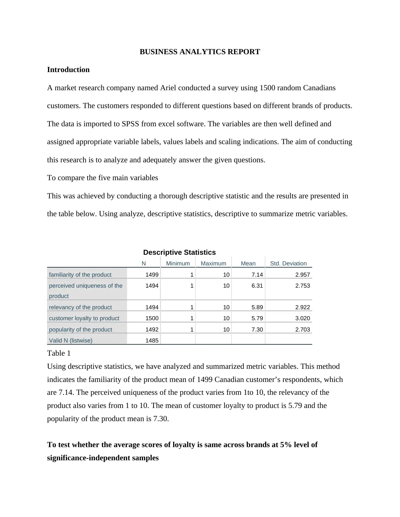
To compare the five main variables
This was achieved by conducting a thorough descriptive statistic and the results are presented in
the table below. Using analyze, descriptive statistics, descriptive to summarize metric variables.
Descriptive Statistics
N Minimum Maximum Mean Std. Deviation
familiarity of the product 1499 1 10 7.14 2.957
perceived uniqueness of the
product
1494 1 10 6.31 2.753
relevancy of the product 1494 1 10 5.89 2.922
customer loyalty to product 1500 1 10 5.79 3.020
popularity of the product 1492 1 10 7.30 2.703
Valid N (listwise) 1485
Table 1
Using descriptive statistics, we have analyzed and summarized metric variables. This method
indicates the familiarity of the product mean of 1499 Canadian customer’s respondents, which
are 7.14. The perceived uniqueness of the product varies from 1to 10, the relevancy of the
product also varies from 1 to 10. The mean of customer loyalty to product is 5.79 and the
popularity of the product mean is 7.30.
To test whether the average scores of loyalty is same across brands at 5% level of
significance-independent samples
Paraphrase This Document
Need a fresh take? Get an instant paraphrase of this document with our AI Paraphraser
Group Statistics
brand N Mean Std. Deviation Std. Error Mean
customer loyalty to product Brand 1 283 5.80 2.767 .164
Brand 2 291 5.59 3.030 .178
Independent Samples Tes
Levene's Test for Equality of Variances
F Sig. t df
customer loyalty to product Equal variances assumed 7.144 .008 .871
Equal variances not assumed .872 569
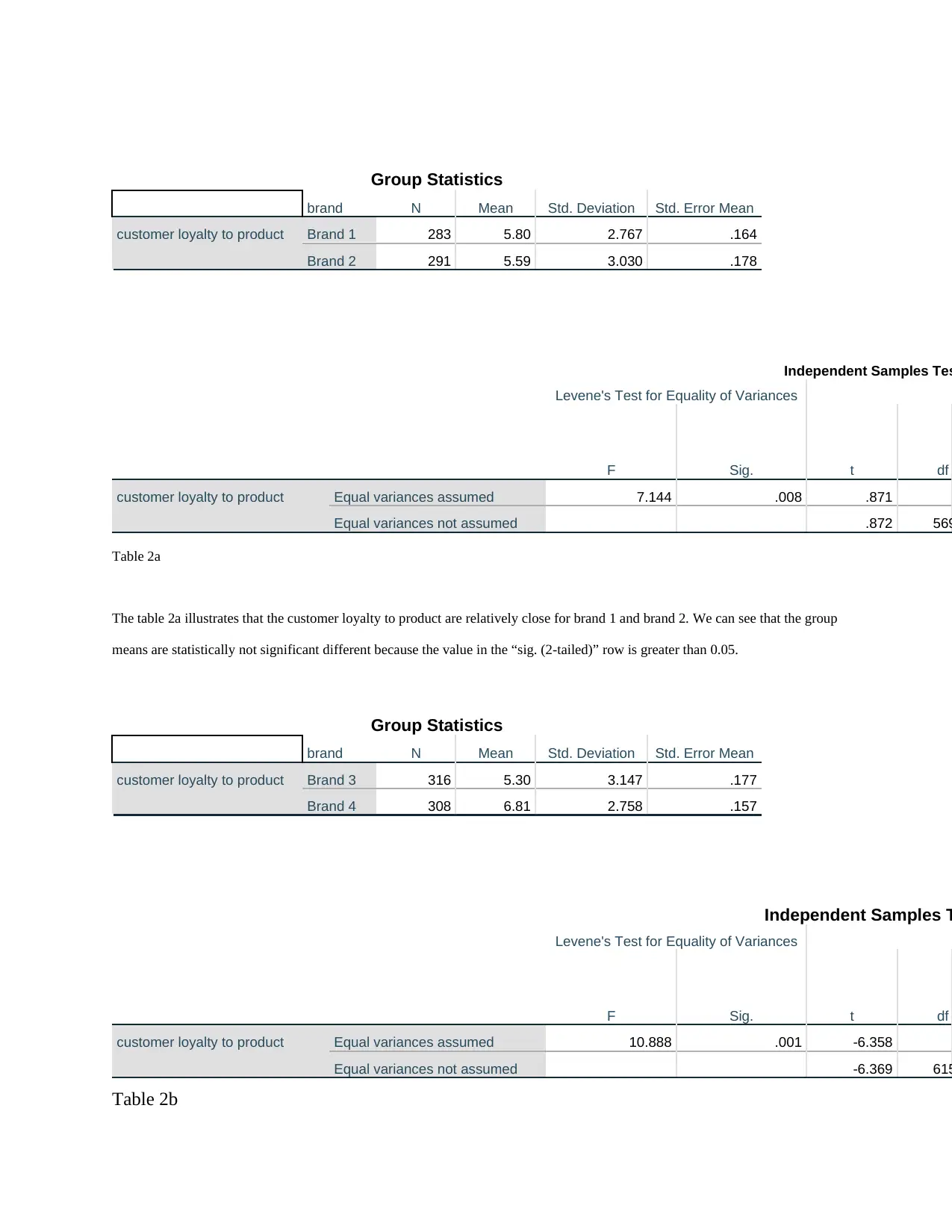
Table 2a
The table 2a illustrates that the customer loyalty to product are relatively close for brand 1 and brand 2. We can see that the group
means are statistically not significant different because the value in the “sig. (2-tailed)” row is greater than 0.05.
Group Statistics
brand N Mean Std. Deviation Std. Error Mean
customer loyalty to product Brand 3 316 5.30 3.147 .177
Brand 4 308 6.81 2.758 .157
Independent Samples T
Levene's Test for Equality of Variances
F Sig. t df
customer loyalty to product Equal variances assumed 10.888 .001 -6.358
Equal variances not assumed -6.369 615
Table 2b
brand N Mean Std. Deviation Std. Error Mean
customer loyalty to product Brand 1 283 5.80 2.767 .164
Brand 2 291 5.59 3.030 .178
Independent Samples Tes
Levene's Test for Equality of Variances
F Sig. t df
customer loyalty to product Equal variances assumed 7.144 .008 .871
Equal variances not assumed .872 569
Table 2a
The table 2a illustrates that the customer loyalty to product are relatively close for brand 1 and brand 2. We can see that the group
means are statistically not significant different because the value in the “sig. (2-tailed)” row is greater than 0.05.
Group Statistics
brand N Mean Std. Deviation Std. Error Mean
customer loyalty to product Brand 3 316 5.30 3.147 .177
Brand 4 308 6.81 2.758 .157
Independent Samples T
Levene's Test for Equality of Variances
F Sig. t df
customer loyalty to product Equal variances assumed 10.888 .001 -6.358
Equal variances not assumed -6.369 615
Table 2b
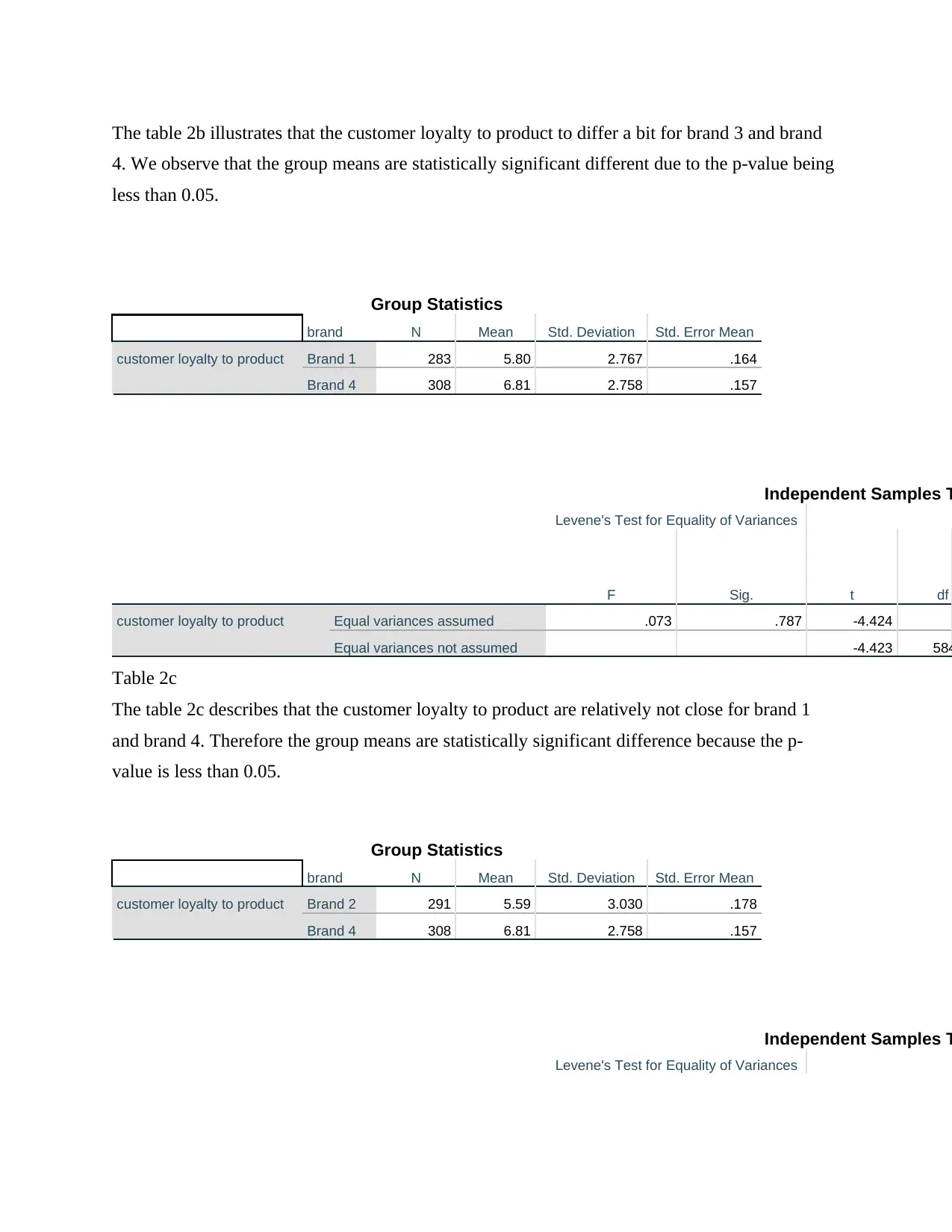
The table 2b illustrates that the customer loyalty to product to differ a bit for brand 3 and brand
4. We observe that the group means are statistically significant different due to the p-value being
less than 0.05.
Group Statistics
brand N Mean Std. Deviation Std. Error Mean
customer loyalty to product Brand 1 283 5.80 2.767 .164
Brand 4 308 6.81 2.758 .157
Independent Samples T
Levene's Test for Equality of Variances
F Sig. t df
customer loyalty to product Equal variances assumed .073 .787 -4.424
Equal variances not assumed -4.423 584
Table 2c
The table 2c describes that the customer loyalty to product are relatively not close for brand 1
and brand 4. Therefore the group means are statistically significant difference because the p-
value is less than 0.05.
Group Statistics
brand N Mean Std. Deviation Std. Error Mean
customer loyalty to product Brand 2 291 5.59 3.030 .178
Brand 4 308 6.81 2.758 .157
Independent Samples T
Levene's Test for Equality of Variances
⊘ This is a preview!⊘
Do you want full access?
Subscribe today to unlock all pages.

Trusted by 1+ million students worldwide
F Sig. t df
customer loyalty to product Equal variances assumed 6.328 .012 -5.147
Equal variances not assumed -5.133 583
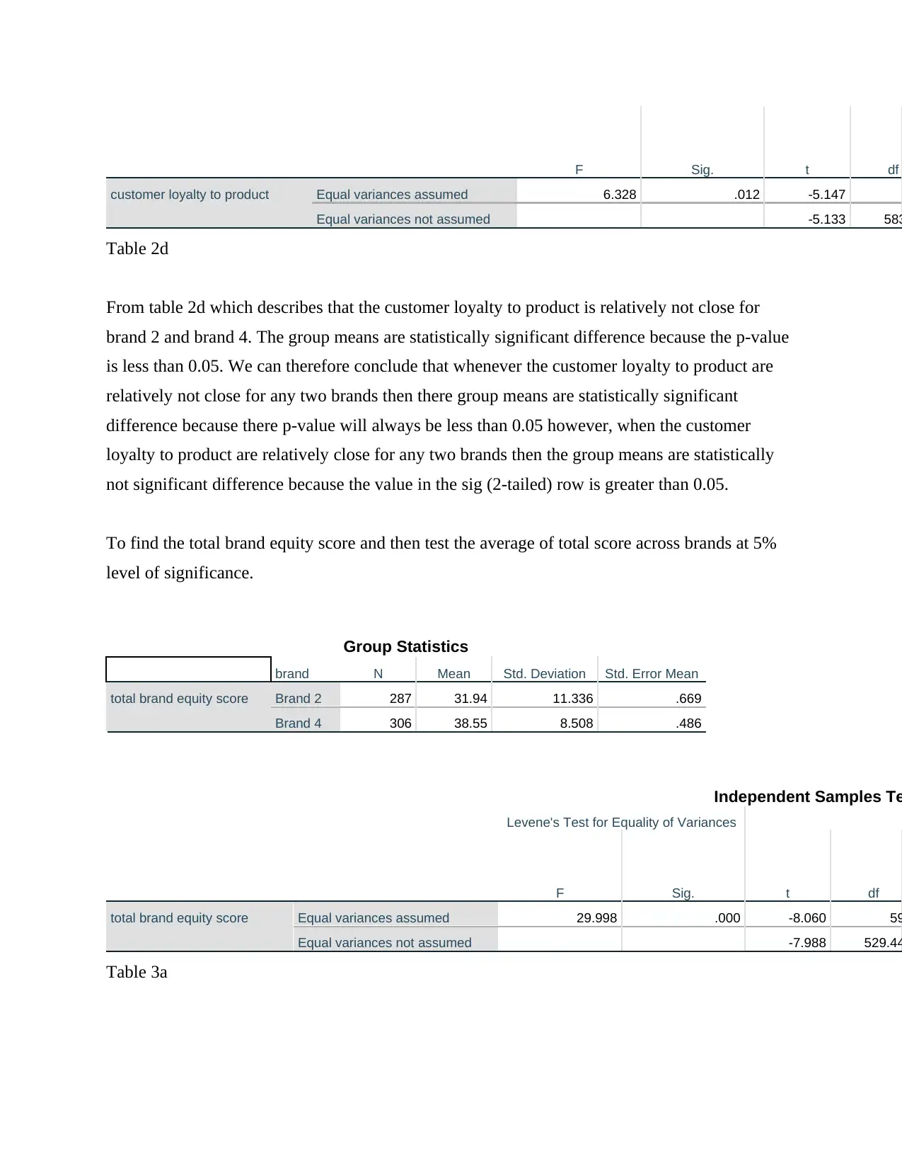
Table 2d
From table 2d which describes that the customer loyalty to product is relatively not close for
brand 2 and brand 4. The group means are statistically significant difference because the p-value
is less than 0.05. We can therefore conclude that whenever the customer loyalty to product are
relatively not close for any two brands then there group means are statistically significant
difference because there p-value will always be less than 0.05 however, when the customer
loyalty to product are relatively close for any two brands then the group means are statistically
not significant difference because the value in the sig (2-tailed) row is greater than 0.05.
To find the total brand equity score and then test the average of total score across brands at 5%
level of significance.
Group Statistics
brand N Mean Std. Deviation Std. Error Mean
total brand equity score Brand 2 287 31.94 11.336 .669
Brand 4 306 38.55 8.508 .486
Independent Samples Te
Levene's Test for Equality of Variances
F Sig. t df
total brand equity score Equal variances assumed 29.998 .000 -8.060 59
Equal variances not assumed -7.988 529.44
Table 3a
Paraphrase This Document
Need a fresh take? Get an instant paraphrase of this document with our AI Paraphraser
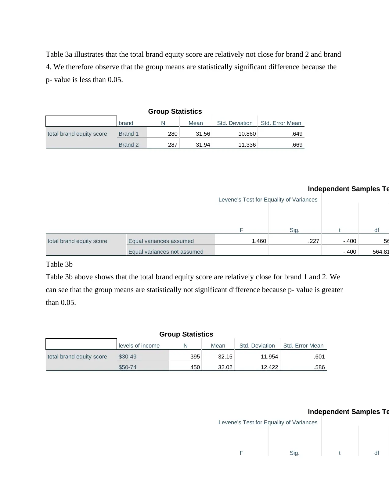
Table 3a illustrates that the total brand equity score are relatively not close for brand 2 and brand
4. We therefore observe that the group means are statistically significant difference because the
p- value is less than 0.05.
Group Statistics
brand N Mean Std. Deviation Std. Error Mean
total brand equity score Brand 1 280 31.56 10.860 .649
Brand 2 287 31.94 11.336 .669
Independent Samples Te
Levene's Test for Equality of Variances
F Sig. t df
total brand equity score Equal variances assumed 1.460 .227 -.400 56
Equal variances not assumed -.400 564.81
Table 3b
Table 3b above shows that the total brand equity score are relatively close for brand 1 and 2. We
can see that the group means are statistically not significant difference because p- value is greater
than 0.05.
Group Statistics
levels of income N Mean Std. Deviation Std. Error Mean
total brand equity score $30-49 395 32.15 11.954 .601
$50-74 450 32.02 12.422 .586
Independent Samples Te
Levene's Test for Equality of Variances
F Sig. t df
total brand equity score Equal variances assumed .696 .405 .154 84
Equal variances not assumed .155 835.89
Table 4a
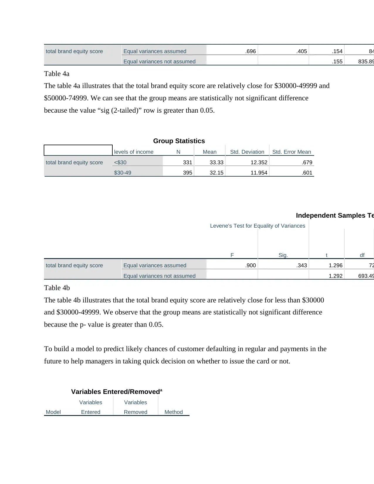
The table 4a illustrates that the total brand equity score are relatively close for $30000-49999 and
$50000-74999. We can see that the group means are statistically not significant difference
because the value “sig (2-tailed)” row is greater than 0.05.
Group Statistics
levels of income N Mean Std. Deviation Std. Error Mean
total brand equity score <$30 331 33.33 12.352 .679
$30-49 395 32.15 11.954 .601
Independent Samples Te
Levene's Test for Equality of Variances
F Sig. t df
total brand equity score Equal variances assumed .900 .343 1.296 72
Equal variances not assumed 1.292 693.49
Table 4b
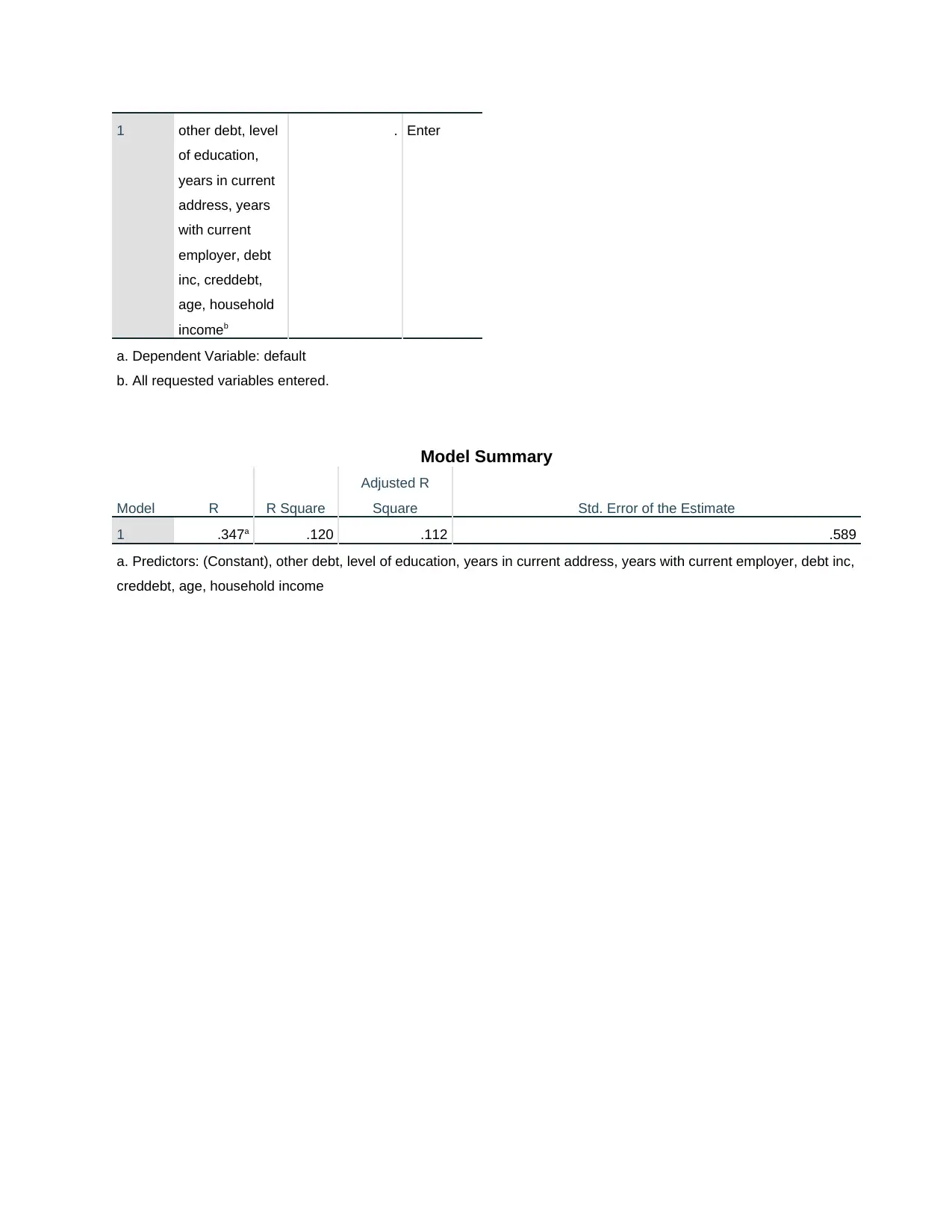
The table 4b illustrates that the total brand equity score are relatively close for less than $30000
and $30000-49999. We observe that the group means are statistically not significant difference
because the p- value is greater than 0.05.
To build a model to predict likely chances of customer defaulting in regular and payments in the
future to help managers in taking quick decision on whether to issue the card or not.
Variables Entered/Removeda
Model
Variables
Entered
Variables
Removed Method
⊘ This is a preview!⊘
Do you want full access?
Subscribe today to unlock all pages.

Trusted by 1+ million students worldwide
1 other debt, level
of education,
years in current
address, years
with current
employer, debt
inc, creddebt,
age, household
incomeb
. Enter
a. Dependent Variable: default
b. All requested variables entered.
Model Summary
Model R R Square
Adjusted R
Square Std. Error of the Estimate
1 .347a .120 .112 .589
a. Predictors: (Constant), other debt, level of education, years in current address, years with current employer, debt inc,
creddebt, age, household income
Paraphrase This Document
Need a fresh take? Get an instant paraphrase of this document with our AI Paraphraser
ANOVAa
Model Sum of Squares df Mean Square F Sig.
1 Regression 39.847 8 4.981 14.352 .000b
Residual 291.872 841 .347
Total 331.719 849
a. Dependent Variable: default
b. Predictors: (Constant), other debt, level of education, years in current address, years with
current employer, debt inc, creddebt, age, household income
Coefficientsa
Model
Unstandardized Coefficients
Standardized
Coefficients
t Sig.B Std. Error Beta
1 (Constant) 1.848 .124 14.887 .000
age .001 .004 .013 .278 .781
level of education .049 .020 .081 2.437 .015
years with current employer -.020 .004 -.220 -4.816 .000
years in current address -.006 .004 -.062 -1.528 .127
household income .001 .001 .033 .526 .599
debt inc .020 .005 .217 3.856 .000
creddebt .035 .015 .120 2.354 .019
other debt -.012 .011 -.063 -1.023 .307
a. Dependent Variable: default
Table 5
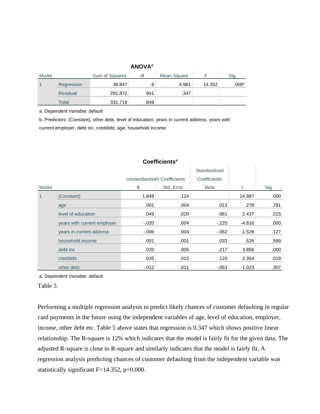
Performing a multiple regression analysis to predict likely chances of customer defaulting in regular
card payments in the future using the independent variables of age, level of education, employer,
income, other debt etc. Table 5 above states that regression is 0.347 which shows positive linear
relationship. The R-square is 12% which indicates that the model is fairly fit for the given data. The
adjusted R-square is close to R-square and similarly indicates that the model is fairly fit. A
regression analysis predicting chances of customer defaulting from the independent variable was
statistically significant F=14.352, p=0.000.
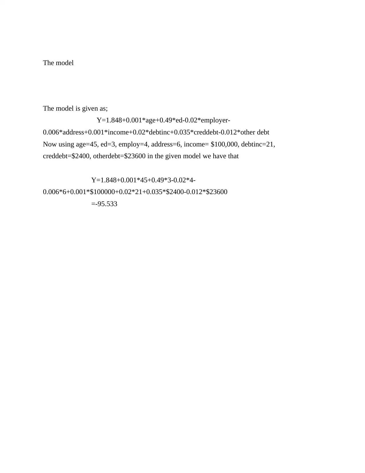
The model
The model is given as;
Y=1.848+0.001*age+0.49*ed-0.02*employer-
0.006*address+0.001*income+0.02*debtinc+0.035*creddebt-0.012*other debt
Now using age=45, ed=3, employ=4, address=6, income= $100,000, debtinc=21,
creddebt=$2400, otherdebt=$23600 in the given model we have that
Y=1.848+0.001*45+0.49*3-0.02*4-
0.006*6+0.001*$100000+0.02*21+0.035*$2400-0.012*$23600
=-95.533
⊘ This is a preview!⊘
Do you want full access?
Subscribe today to unlock all pages.

Trusted by 1+ million students worldwide
1 out of 9
Related Documents
Your All-in-One AI-Powered Toolkit for Academic Success.
+13062052269
info@desklib.com
Available 24*7 on WhatsApp / Email
![[object Object]](/_next/static/media/star-bottom.7253800d.svg)
Unlock your academic potential
Copyright © 2020–2026 A2Z Services. All Rights Reserved. Developed and managed by ZUCOL.


