Marks intervals Business Data Analysis 2022
VerifiedAdded on 2022/08/28
|11
|1099
|11
AI Summary
Contribute Materials
Your contribution can guide someone’s learning journey. Share your
documents today.
Running head: BUSINESS DATA ANALYSIS
BUSINESS DATA ANALYSIS
Name of the Student
Name of the University
Author Note
BUSINESS DATA ANALYSIS
Name of the Student
Name of the University
Author Note
Secure Best Marks with AI Grader
Need help grading? Try our AI Grader for instant feedback on your assignments.
1BUSINESS DATA ANALYSIS
Question 1:
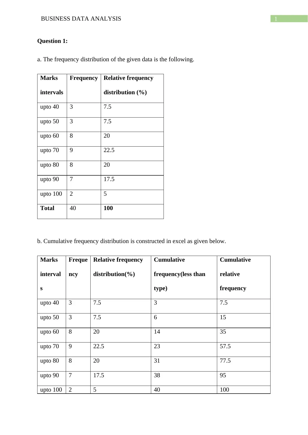
a. The frequency distribution of the given data is the following.
Marks
intervals
Frequency Relative frequency
distribution (%)
upto 40 3 7.5
upto 50 3 7.5
upto 60 8 20
upto 70 9 22.5
upto 80 8 20
upto 90 7 17.5
upto 100 2 5
Total 40 100
b. Cumulative frequency distribution is constructed in excel as given below.
Marks
interval
s
Freque
ncy
Relative frequency
distribution(%)
Cumulative
frequency(less than
type)
Cumulative
relative
frequency
upto 40 3 7.5 3 7.5
upto 50 3 7.5 6 15
upto 60 8 20 14 35
upto 70 9 22.5 23 57.5
upto 80 8 20 31 77.5
upto 90 7 17.5 38 95
upto 100 2 5 40 100
Question 1:
a. The frequency distribution of the given data is the following.
Marks
intervals
Frequency Relative frequency
distribution (%)
upto 40 3 7.5
upto 50 3 7.5
upto 60 8 20
upto 70 9 22.5
upto 80 8 20
upto 90 7 17.5
upto 100 2 5
Total 40 100
b. Cumulative frequency distribution is constructed in excel as given below.
Marks
interval
s
Freque
ncy
Relative frequency
distribution(%)
Cumulative
frequency(less than
type)
Cumulative
relative
frequency
upto 40 3 7.5 3 7.5
upto 50 3 7.5 6 15
upto 60 8 20 14 35
upto 70 9 22.5 23 57.5
upto 80 8 20 31 77.5
upto 90 7 17.5 38 95
upto 100 2 5 40 100
2BUSINESS DATA ANALYSIS
Total 40 100
c. Relative frequency histogram is the histogram of relative frequency of each class or
interval in percentage.
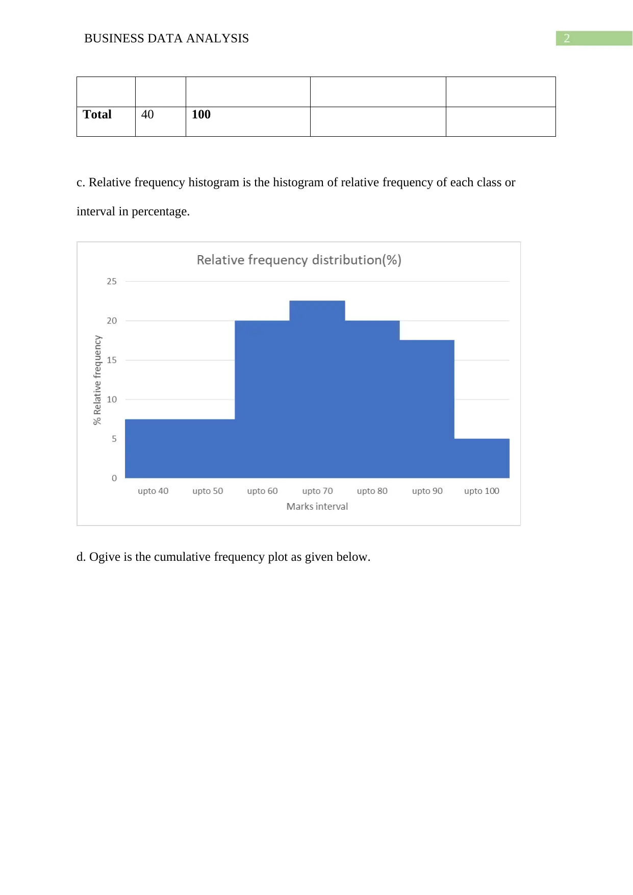
d. Ogive is the cumulative frequency plot as given below.
Total 40 100
c. Relative frequency histogram is the histogram of relative frequency of each class or
interval in percentage.
d. Ogive is the cumulative frequency plot as given below.
3BUSINESS DATA ANALYSIS
e. The count of marks which is less than or equal to 60 is obtained from the Ogive which is
14. Hence, the required proportion = 14/total frequency = 14/40 = 0.35 or 35%.
f. The count of marks which is less than or equal to 70 is 23. Hence, the required proportion =
23/40 = 0.575 = 57.5%
Question 2:
Total number of 18 years or older people moved = 1494 thousand.
Moved for housing reasons = 758.2 thousand
Moved for employment reasons = 170.2 thousand
Moved for family reasons = 398.6 thousand
Moved for other reasons = 167.2 thousand
Summarized in the following table.
Secure Best Marks with AI Grader
Need help grading? Try our AI Grader for instant feedback on your assignments.
4BUSINESS DATA ANALYSIS
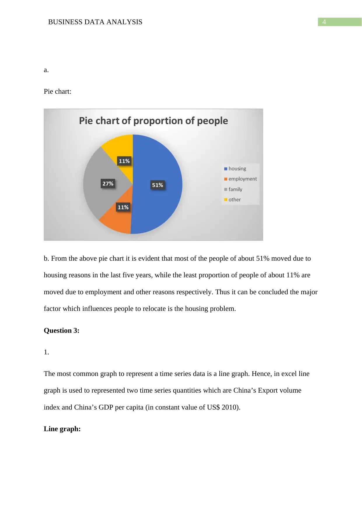
a.
Pie chart:
b. From the above pie chart it is evident that most of the people of about 51% moved due to
housing reasons in the last five years, while the least proportion of people of about 11% are
moved due to employment and other reasons respectively. Thus it can be concluded the major
factor which influences people to relocate is the housing problem.
Question 3:
1.
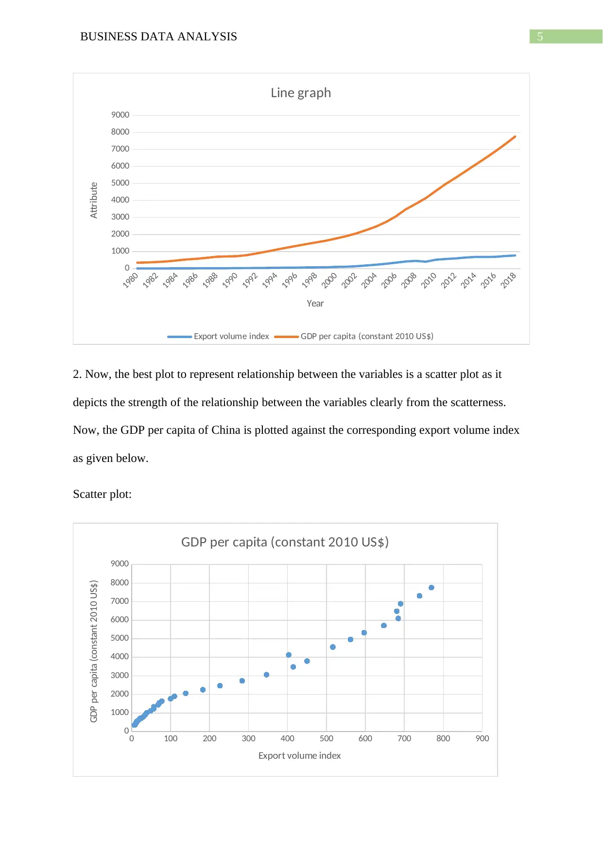
The most common graph to represent a time series data is a line graph. Hence, in excel line
graph is used to represented two time series quantities which are China’s Export volume
index and China’s GDP per capita (in constant value of US$ 2010).
Line graph:
a.
Pie chart:
b. From the above pie chart it is evident that most of the people of about 51% moved due to
housing reasons in the last five years, while the least proportion of people of about 11% are
moved due to employment and other reasons respectively. Thus it can be concluded the major
factor which influences people to relocate is the housing problem.
Question 3:
1.
The most common graph to represent a time series data is a line graph. Hence, in excel line
graph is used to represented two time series quantities which are China’s Export volume
index and China’s GDP per capita (in constant value of US$ 2010).
Line graph:
5BUSINESS DATA ANALYSIS
1980
1982
1984
1986
1988
1990
1992
1994
1996
1998
2000
2002
2004
2006
2008
2010
2012
2014
2016
2018
0
1000
2000
3000
4000
5000
6000
7000
8000
9000
Line graph
Export volume index GDP per capita (constant 2010 US$)
Year
Attribute
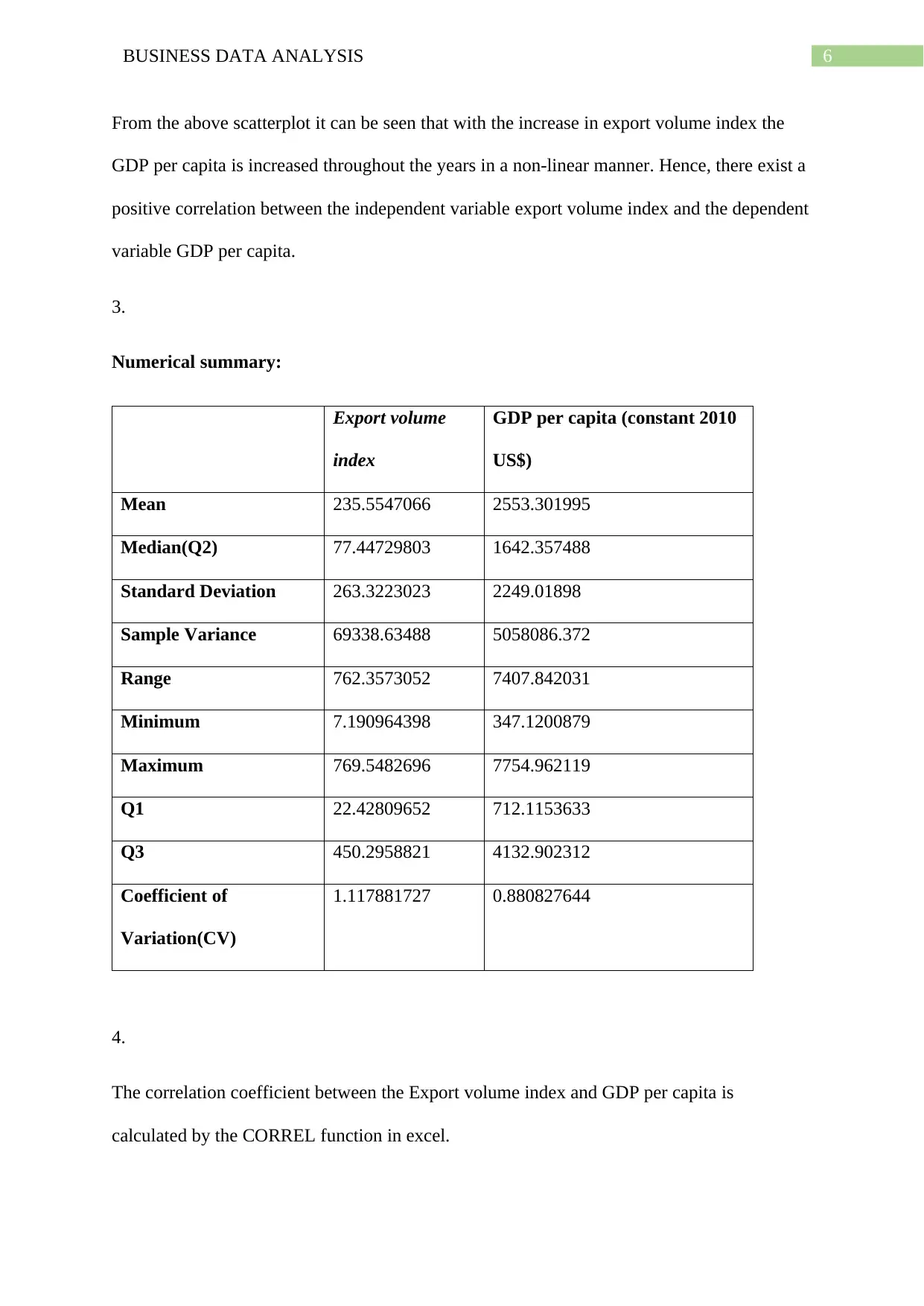
2. Now, the best plot to represent relationship between the variables is a scatter plot as it
depicts the strength of the relationship between the variables clearly from the scatterness.
Now, the GDP per capita of China is plotted against the corresponding export volume index
as given below.
Scatter plot:
0 100 200 300 400 500 600 700 800 900
0
1000
2000
3000
4000
5000
6000
7000
8000
9000
GDP per capita (constant 2010 US$)
Export volume index
GDP per capita (constant 2010 US$)
1980
1982
1984
1986
1988
1990
1992
1994
1996
1998
2000
2002
2004
2006
2008
2010
2012
2014
2016
2018
0
1000
2000
3000
4000
5000
6000
7000
8000
9000
Line graph
Export volume index GDP per capita (constant 2010 US$)
Year
Attribute
2. Now, the best plot to represent relationship between the variables is a scatter plot as it
depicts the strength of the relationship between the variables clearly from the scatterness.
Now, the GDP per capita of China is plotted against the corresponding export volume index
as given below.
Scatter plot:
0 100 200 300 400 500 600 700 800 900
0
1000
2000
3000
4000
5000
6000
7000
8000
9000
GDP per capita (constant 2010 US$)
Export volume index
GDP per capita (constant 2010 US$)
6BUSINESS DATA ANALYSIS
From the above scatterplot it can be seen that with the increase in export volume index the
GDP per capita is increased throughout the years in a non-linear manner. Hence, there exist a
positive correlation between the independent variable export volume index and the dependent
variable GDP per capita.
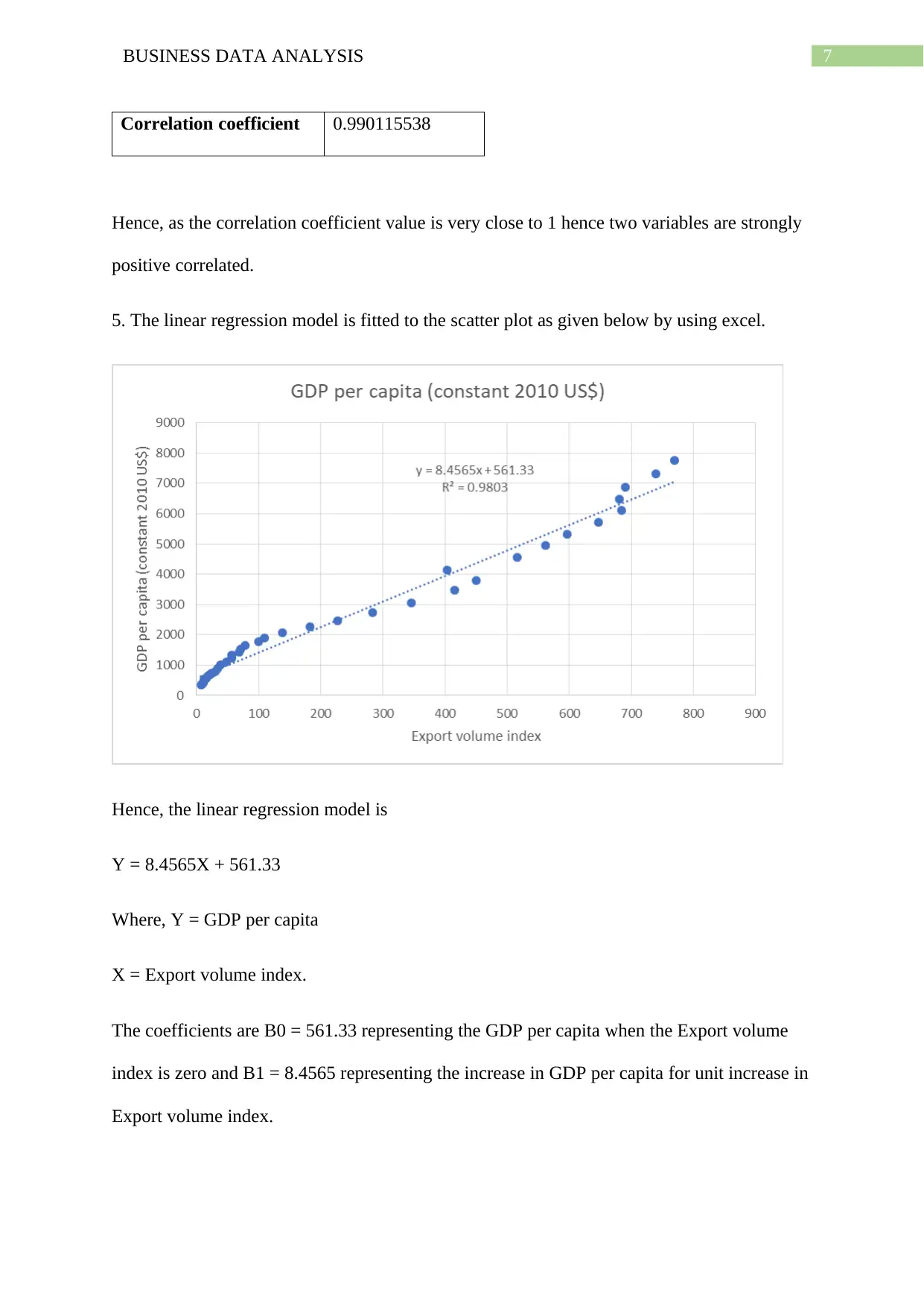
3.
Numerical summary:
Export volume
index
GDP per capita (constant 2010
US$)
Mean 235.5547066 2553.301995
Median(Q2) 77.44729803 1642.357488
Standard Deviation 263.3223023 2249.01898
Sample Variance 69338.63488 5058086.372
Range 762.3573052 7407.842031
Minimum 7.190964398 347.1200879
Maximum 769.5482696 7754.962119
Q1 22.42809652 712.1153633
Q3 450.2958821 4132.902312
Coefficient of
Variation(CV)
1.117881727 0.880827644
4.
The correlation coefficient between the Export volume index and GDP per capita is
calculated by the CORREL function in excel.
From the above scatterplot it can be seen that with the increase in export volume index the
GDP per capita is increased throughout the years in a non-linear manner. Hence, there exist a
positive correlation between the independent variable export volume index and the dependent
variable GDP per capita.
3.
Numerical summary:
Export volume
index
GDP per capita (constant 2010
US$)
Mean 235.5547066 2553.301995
Median(Q2) 77.44729803 1642.357488
Standard Deviation 263.3223023 2249.01898
Sample Variance 69338.63488 5058086.372
Range 762.3573052 7407.842031
Minimum 7.190964398 347.1200879
Maximum 769.5482696 7754.962119
Q1 22.42809652 712.1153633
Q3 450.2958821 4132.902312
Coefficient of
Variation(CV)
1.117881727 0.880827644
4.
The correlation coefficient between the Export volume index and GDP per capita is
calculated by the CORREL function in excel.
Paraphrase This Document
Need a fresh take? Get an instant paraphrase of this document with our AI Paraphraser
7BUSINESS DATA ANALYSIS
Correlation coefficient 0.990115538
Hence, as the correlation coefficient value is very close to 1 hence two variables are strongly
positive correlated.
5. The linear regression model is fitted to the scatter plot as given below by using excel.
Hence, the linear regression model is
Y = 8.4565X + 561.33
Where, Y = GDP per capita
X = Export volume index.
The coefficients are B0 = 561.33 representing the GDP per capita when the Export volume
index is zero and B1 = 8.4565 representing the increase in GDP per capita for unit increase in
Export volume index.
8BUSINESS DATA ANALYSIS
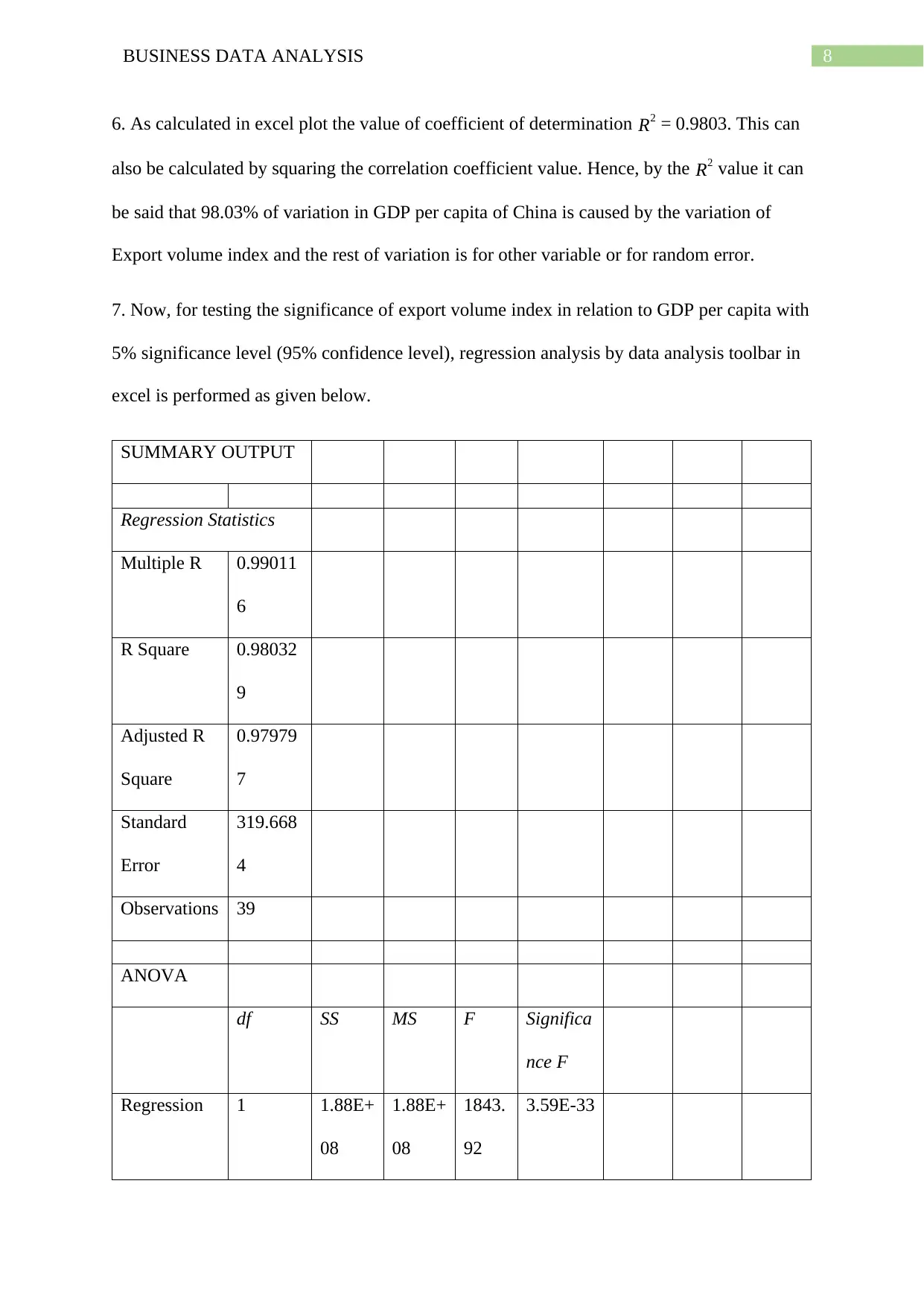
6. As calculated in excel plot the value of coefficient of determination R2 = 0.9803. This can
also be calculated by squaring the correlation coefficient value. Hence, by the R2 value it can
be said that 98.03% of variation in GDP per capita of China is caused by the variation of
Export volume index and the rest of variation is for other variable or for random error.
7. Now, for testing the significance of export volume index in relation to GDP per capita with
5% significance level (95% confidence level), regression analysis by data analysis toolbar in
excel is performed as given below.
SUMMARY OUTPUT
Regression Statistics
Multiple R 0.99011
6
R Square 0.98032
9
Adjusted R
Square
0.97979
7
Standard
Error
319.668
4
Observations 39
ANOVA
df SS MS F Significa
nce F
Regression 1 1.88E+
08
1.88E+
08
1843.
92
3.59E-33
9BUSINESS DATA ANALYSIS
Residual 37 37809
52
10218
7.9
Total 38 1.92E+
08
Coeffici
ents
Standa
rd
Error
t Stat P-
value
Lower
95%
Upper
95%
Lower
95.0%
Upper
95.0%
Intercept 561.330
4
69.080
48
8.1257
46
9.5E-
10
421.360
1
701.30
08
421.36
01
701.30
08
Export
volume
index
8.45651
4
0.1969
34
42.940
89
3.59E
-33
8.05748
8
8.8555
39
8.0574
88
8.8555
39
It can be seen from the table that at 95% confidence or at 5% significance level the export
volume index is positive and has the p value less than 0.05 (significance level). Thus it can be
concluded that GDP per capita is positively and significantly increases with export volume
index.
8. The standard error of estimate is basically the square root of average squared error. This is
given by,
SE = √ 1
N ∑
i=1
N
( Yi− yi ) 2
Here, Yi = estimate values of GDP per capita at given export volume index and yi = Given
value of GDP per capita.
Secure Best Marks with AI Grader
Need help grading? Try our AI Grader for instant feedback on your assignments.
10BUSINESS DATA ANALYSIS
The SE is calculated by STEYX function in excel as 319.6684.
The SE is large and thus indicates that the sample mean is less accurate to the population
mean. This is because the number of given observations is low which is 39. Thus with this
low observations the fitted linear regression model is not a very good fit to GDP per capita vs
export volume index data.
1 out of 11
Related Documents


Your All-in-One AI-Powered Toolkit for Academic Success.
+13062052269
info@desklib.com
Available 24*7 on WhatsApp / Email
![[object Object]](/_next/static/media/star-bottom.7253800d.svg)
Unlock your academic potential
© 2024 | Zucol Services PVT LTD | All rights reserved.