Business Data Analysis - Desklib

This article discusses the use of correlation coefficient and regression model in business data analysis. It explains how to estimate sales level in the 13th quarter and how to determine the fit of a least square line. It also offers an explanation for an aberration in crop yield despite high rainfall. References are provided for further reading.

BUSINESS DATA ANALYSIS
STUDENT ID:
[Pick the date]

Question 1
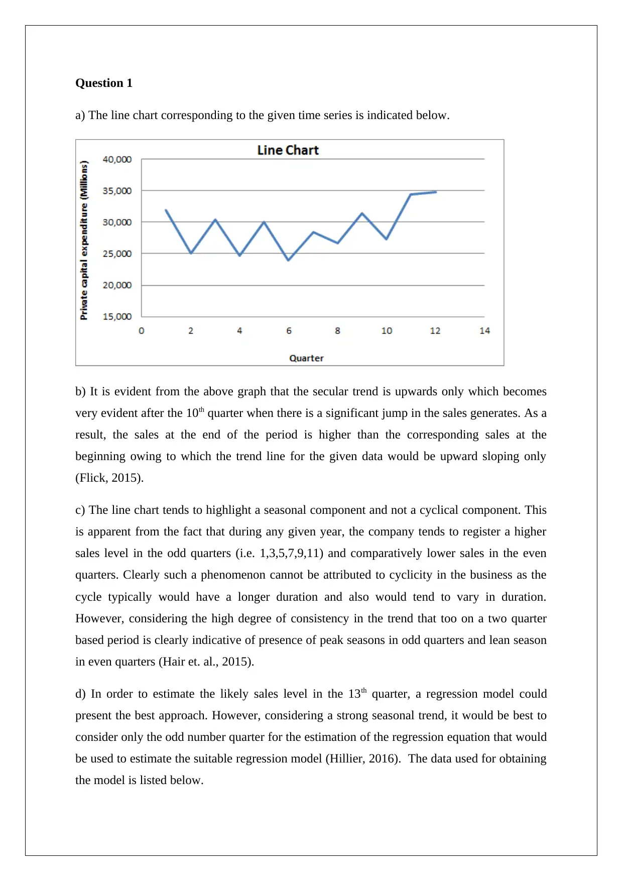
a) The line chart corresponding to the given time series is indicated below.
b) It is evident from the above graph that the secular trend is upwards only which becomes
very evident after the 10th quarter when there is a significant jump in the sales generates. As a
result, the sales at the end of the period is higher than the corresponding sales at the
beginning owing to which the trend line for the given data would be upward sloping only
(Flick, 2015).
c) The line chart tends to highlight a seasonal component and not a cyclical component. This
is apparent from the fact that during any given year, the company tends to register a higher
sales level in the odd quarters (i.e. 1,3,5,7,9,11) and comparatively lower sales in the even
quarters. Clearly such a phenomenon cannot be attributed to cyclicity in the business as the
cycle typically would have a longer duration and also would tend to vary in duration.
However, considering the high degree of consistency in the trend that too on a two quarter
based period is clearly indicative of presence of peak seasons in odd quarters and lean season
in even quarters (Hair et. al., 2015).
d) In order to estimate the likely sales level in the 13th quarter, a regression model could
present the best approach. However, considering a strong seasonal trend, it would be best to
consider only the odd number quarter for the estimation of the regression equation that would
be used to estimate the suitable regression model (Hillier, 2016). The data used for obtaining
the model is listed below.

ODD
quarters
Million
s
1 31,920
2 30,350
3 30,090
4 28,450
5 31,380
6 34,380
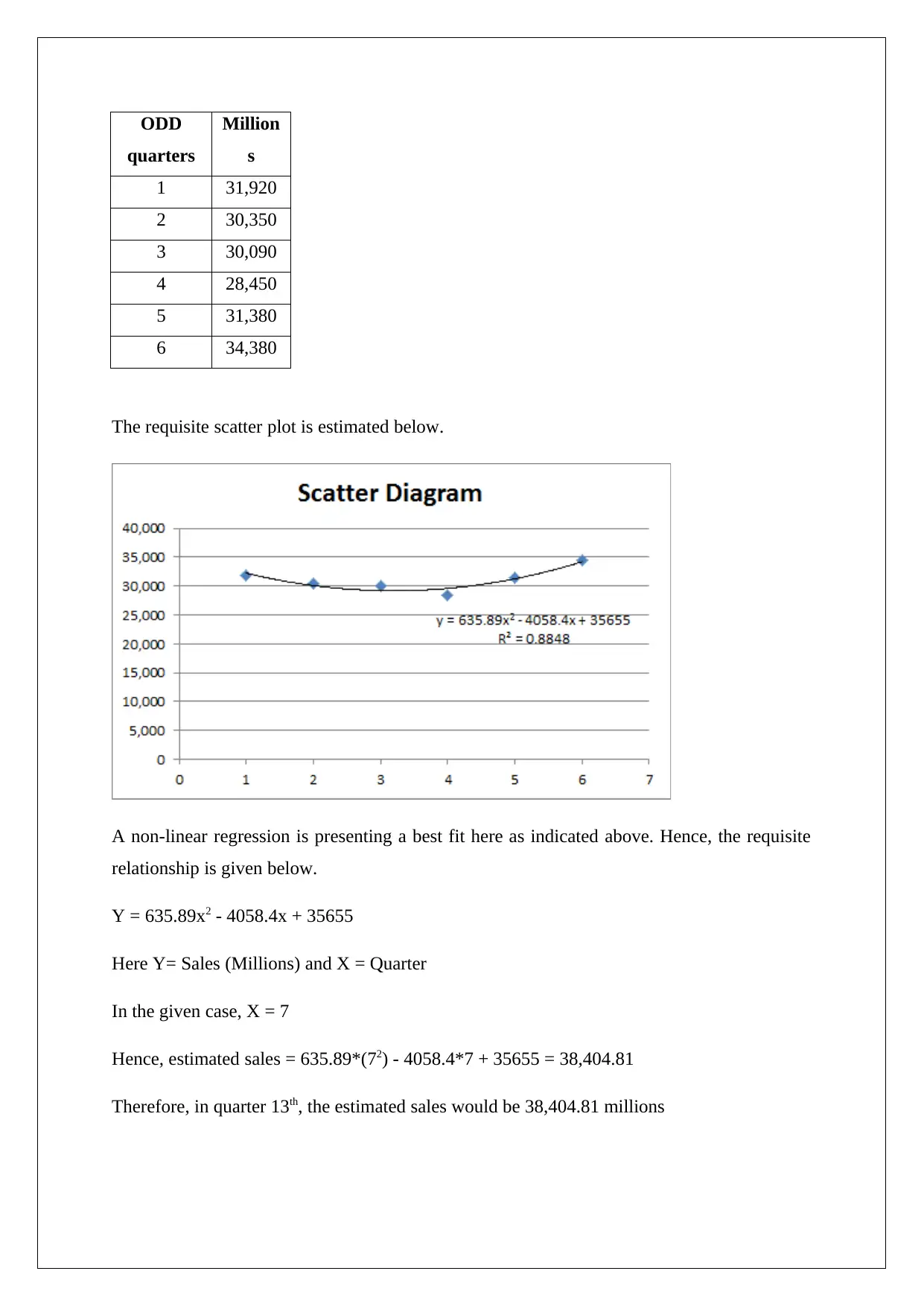
The requisite scatter plot is estimated below.
A non-linear regression is presenting a best fit here as indicated above. Hence, the requisite
relationship is given below.
Y = 635.89x2 - 4058.4x + 35655
Here Y= Sales (Millions) and X = Quarter
In the given case, X = 7
Hence, estimated sales = 635.89*(72) - 4058.4*7 + 35655 = 38,404.81
Therefore, in quarter 13th, the estimated sales would be 38,404.81 millions

Question 2
a) The appropriate measure in order to highlight linear relationship between the given
variables would be correlation coefficient. Taking the given data into consideration, the
correlation coefficient has come out as 0.23. The fact that the correlation coefficient is
positive implies that the nature of the given relationship is positive which implies that the two
variables are more likely to move in the same direction than opposite directions. Also, the
magnitude of the correlation coefficient highlights that the amount of correlation between the
given variables is weak at best (Eriksson and Kovalainen, 2015).
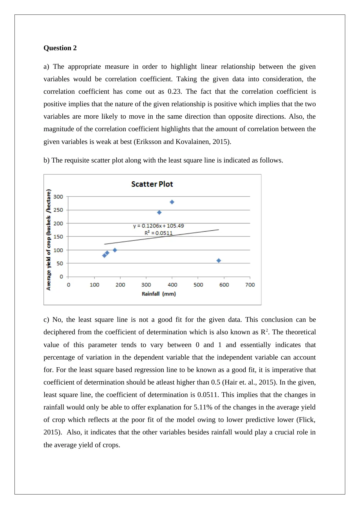
b) The requisite scatter plot along with the least square line is indicated as follows.
c) No, the least square line is not a good fit for the given data. This conclusion can be
deciphered from the coefficient of determination which is also known as R2. The theoretical
value of this parameter tends to vary between 0 and 1 and essentially indicates that
percentage of variation in the dependent variable that the independent variable can account
for. For the least square based regression line to be known as a good fit, it is imperative that
coefficient of determination should be atleast higher than 0.5 (Hair et. al., 2015). In the given,
least square line, the coefficient of determination is 0.0511. This implies that the changes in
rainfall would only be able to offer explanation for 5.11% of the changes in the average yield
of crop which reflects at the poor fit of the model owing to lower predictive lower (Flick,
2015). Also, it indicates that the other variables besides rainfall would play a crucial role in
the average yield of crops.

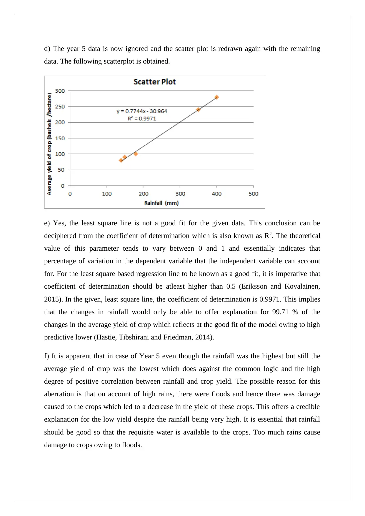
d) The year 5 data is now ignored and the scatter plot is redrawn again with the remaining
data. The following scatterplot is obtained.
e) Yes, the least square line is not a good fit for the given data. This conclusion can be
deciphered from the coefficient of determination which is also known as R2. The theoretical
value of this parameter tends to vary between 0 and 1 and essentially indicates that
percentage of variation in the dependent variable that the independent variable can account
for. For the least square based regression line to be known as a good fit, it is imperative that
coefficient of determination should be atleast higher than 0.5 (Eriksson and Kovalainen,
2015). In the given, least square line, the coefficient of determination is 0.9971. This implies
that the changes in rainfall would only be able to offer explanation for 99.71 % of the
changes in the average yield of crop which reflects at the good fit of the model owing to high
predictive lower (Hastie, Tibshirani and Friedman, 2014).
f) It is apparent that in case of Year 5 even though the rainfall was the highest but still the
average yield of crop was the lowest which does against the common logic and the high
degree of positive correlation between rainfall and crop yield. The possible reason for this
aberration is that on account of high rains, there were floods and hence there was damage
caused to the crops which led to a decrease in the yield of these crops. This offers a credible
explanation for the low yield despite the rainfall being very high. It is essential that rainfall
should be good so that the requisite water is available to the crops. Too much rains cause
damage to crops owing to floods.

References
Eriksson, P. and Kovalainen, A. (2015) Quantitative methods in business research. 3rd ed.
London: Sage Publications.
Flick, U. (2015) Introducing research methodology: A beginner's guide to doing a research
project. 4th ed. New York: Sage Publications.
Hair, J. F., Wolfinbarger, M., Money, A. H., Samouel, P., and Page, M. J. (2015) Essentials
of business research methods. 2nd ed. New York: Routledge.
Hastie, T., Tibshirani, R. and Friedman, J. (2014) The Elements of Statistical Learning. 4th
ed. New York: Springer Publications.
Hillier, F. (2016) Introduction to Operations Research. 6th ed. New York: McGraw Hill
Publications.