Business Decision Making using Statistical Tools
VerifiedAdded on 2022/12/22
|11
|1928
|2
AI Summary
This document discusses the use of statistical tools in business decision making. It explores the impact of exports on different countries and analyzes the correlation between retail turnover and final consumption expenditure. The document also provides numerical summaries and regression analysis for further understanding.
Contribute Materials
Your contribution can guide someone’s learning journey. Share your
documents today.

1
Business Decision Making using Statistical Tools
Business Decision Making using Statistical Tools
Secure Best Marks with AI Grader
Need help grading? Try our AI Grader for instant feedback on your assignments.
2
China Japan United
States Republic of
Korea India New
Zealand Singapore United
Kingdom
0
10
20
30
40
50
60
70
80
90
100
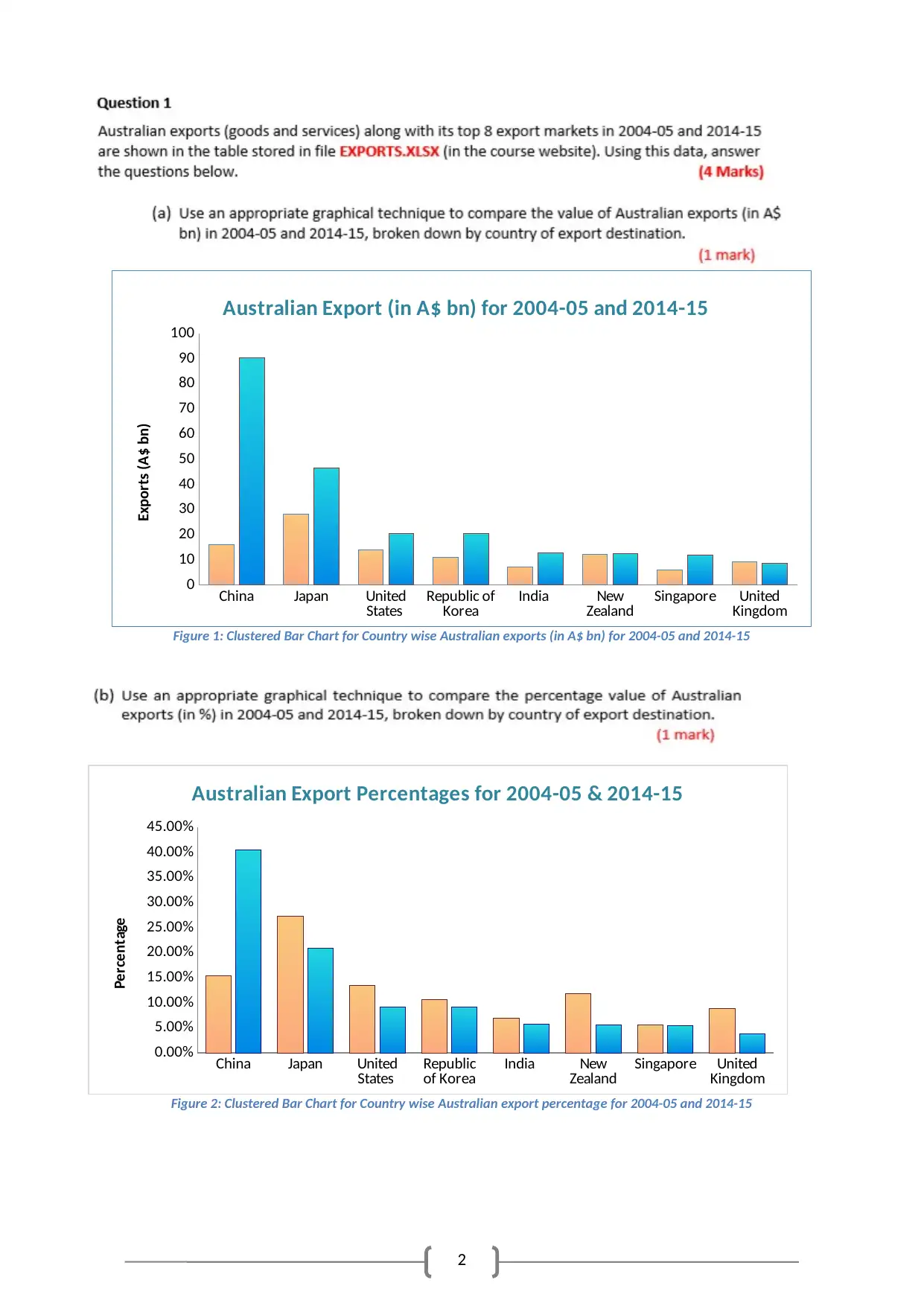
Australian Export (in A$ bn) for 2004-05 and 2014-15
Exports (A$ bn)
Figure 1: Clustered Bar Chart for Country wise Australian exports (in A$ bn) for 2004-05 and 2014-15
China Japan United
States Republic
of Korea India New
Zealand Singapore United
Kingdom
0.00%
5.00%
10.00%
15.00%
20.00%
25.00%
30.00%
35.00%
40.00%
45.00%
Australian Export Percentages for 2004-05 & 2014-15
Percentage
Figure 2: Clustered Bar Chart for Country wise Australian export percentage for 2004-05 and 2014-15
China Japan United
States Republic of
Korea India New
Zealand Singapore United
Kingdom
0
10
20
30
40
50
60
70
80
90
100
Australian Export (in A$ bn) for 2004-05 and 2014-15
Exports (A$ bn)
Figure 1: Clustered Bar Chart for Country wise Australian exports (in A$ bn) for 2004-05 and 2014-15
China Japan United
States Republic
of Korea India New
Zealand Singapore United
Kingdom
0.00%
5.00%
10.00%
15.00%
20.00%
25.00%
30.00%
35.00%
40.00%
45.00%
Australian Export Percentages for 2004-05 & 2014-15
Percentage
Figure 2: Clustered Bar Chart for Country wise Australian export percentage for 2004-05 and 2014-15
3
Exports to China and Japan significantly increased in 2014-15 compared to 2004-05.
Exports to United Kingdom decreased by 0.6 billion Australian dollars, whereas, it
increased to United States, Republic of Korea, India, and Singapore. A very small increase
in exports to New Zealand is also noted.
Exports increased by 25.01% to China, and the impact are felt on the entire scenario.
Exports have decreased by 6.45% to Japan, 4.29%, to the United States, 1.48% to
Republic of Korea, 1.19% to India, and 0.24% to Singapore. A substantial decrease in
exports to New Zealand by 6.31%, and 5.06% to United Kingdom has also been identified
(Triola, 2018).
Interestingly, comparison in export percentages revealed that export to China has grown at
a rapid rate, whereas, percentage export to rest of the countries have decreased. This
indicates that impact of growing trade with China compared to other countries has a
retarding effect on percentage of export to other countries.
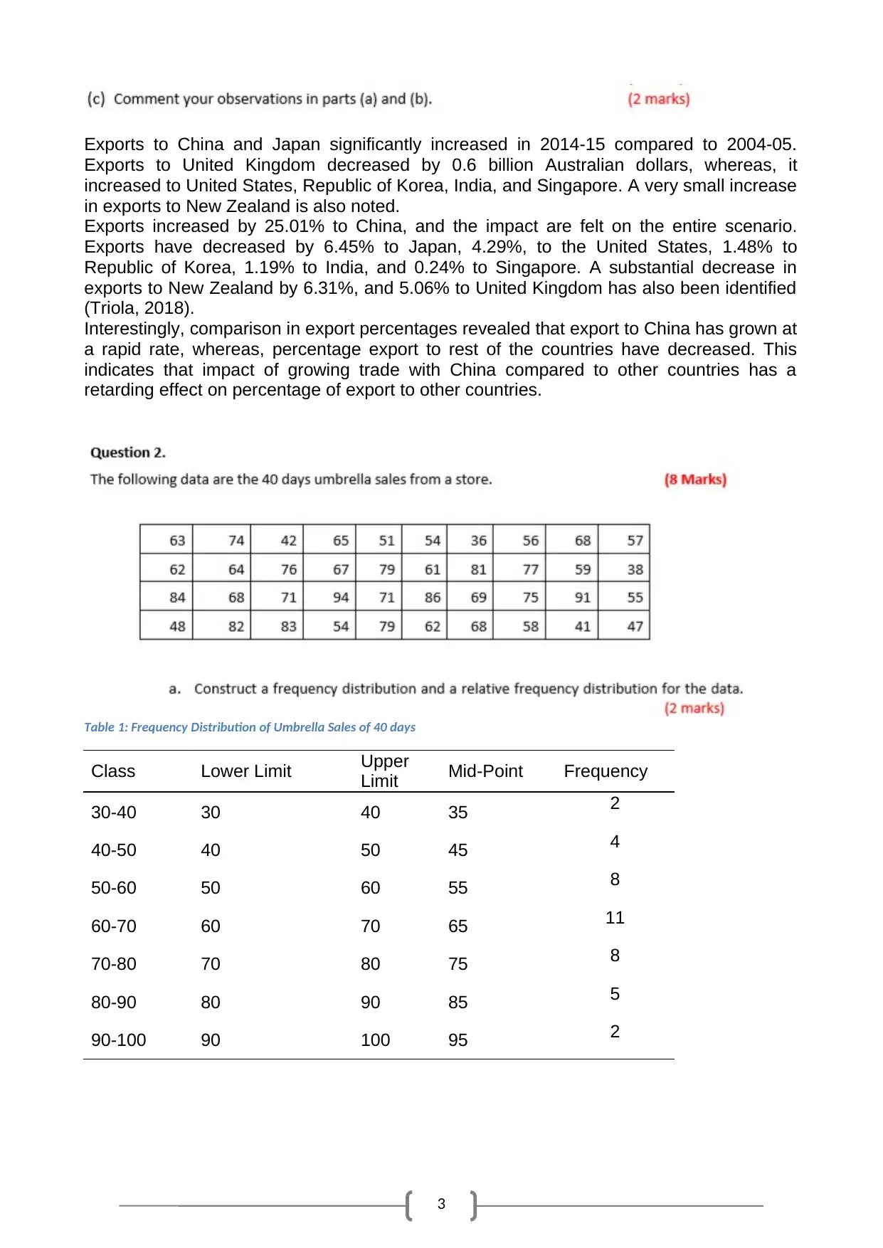
Table 1: Frequency Distribution of Umbrella Sales of 40 days
Class Lower Limit Upper
Limit Mid-Point Frequency
30-40 30 40 35 2
40-50 40 50 45 4
50-60 50 60 55 8
60-70 60 70 65 11
70-80 70 80 75 8
80-90 80 90 85 5
90-100 90 100 95 2
Exports to China and Japan significantly increased in 2014-15 compared to 2004-05.
Exports to United Kingdom decreased by 0.6 billion Australian dollars, whereas, it
increased to United States, Republic of Korea, India, and Singapore. A very small increase
in exports to New Zealand is also noted.
Exports increased by 25.01% to China, and the impact are felt on the entire scenario.
Exports have decreased by 6.45% to Japan, 4.29%, to the United States, 1.48% to
Republic of Korea, 1.19% to India, and 0.24% to Singapore. A substantial decrease in
exports to New Zealand by 6.31%, and 5.06% to United Kingdom has also been identified
(Triola, 2018).
Interestingly, comparison in export percentages revealed that export to China has grown at
a rapid rate, whereas, percentage export to rest of the countries have decreased. This
indicates that impact of growing trade with China compared to other countries has a
retarding effect on percentage of export to other countries.
Table 1: Frequency Distribution of Umbrella Sales of 40 days
Class Lower Limit Upper
Limit Mid-Point Frequency
30-40 30 40 35 2
40-50 40 50 45 4
50-60 50 60 55 8
60-70 60 70 65 11
70-80 70 80 75 8
80-90 80 90 85 5
90-100 90 100 95 2
4
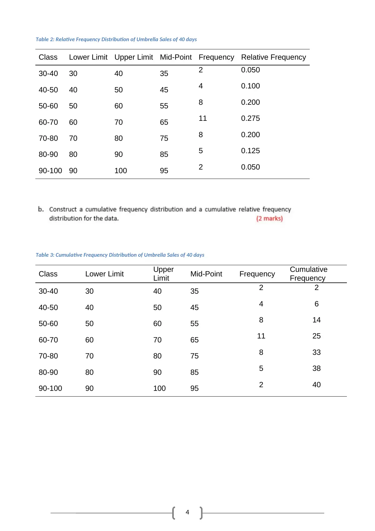
Table 2: Relative Frequency Distribution of Umbrella Sales of 40 days
Class Lower Limit Upper Limit Mid-Point Frequency Relative Frequency
30-40 30 40 35 2 0.050
40-50 40 50 45 4 0.100
50-60 50 60 55 8 0.200
60-70 60 70 65 11 0.275
70-80 70 80 75 8 0.200
80-90 80 90 85 5 0.125
90-100 90 100 95 2 0.050
Table 3: Cumulative Frequency Distribution of Umbrella Sales of 40 days
Class Lower Limit Upper
Limit Mid-Point Frequency Cumulative
Frequency
30-40 30 40 35 2 2
40-50 40 50 45 4 6
50-60 50 60 55 8 14
60-70 60 70 65 11 25
70-80 70 80 75 8 33
80-90 80 90 85 5 38
90-100 90 100 95 2 40
Secure Best Marks with AI Grader
Need help grading? Try our AI Grader for instant feedback on your assignments.
5
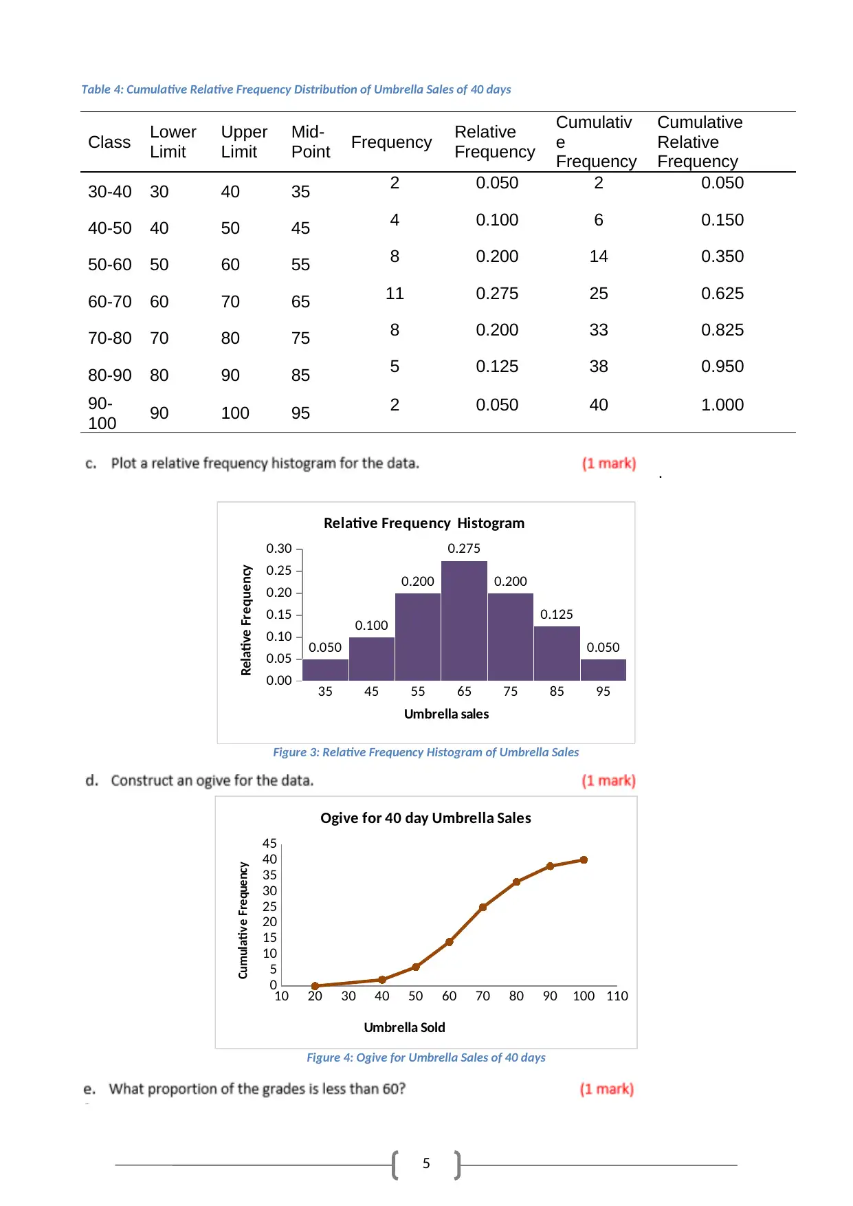
Table 4: Cumulative Relative Frequency Distribution of Umbrella Sales of 40 days
Class Lower
Limit
Upper
Limit
Mid-
Point Frequency Relative
Frequency
Cumulativ
e
Frequency
Cumulative
Relative
Frequency
30-40 30 40 35 2 0.050 2 0.050
40-50 40 50 45 4 0.100 6 0.150
50-60 50 60 55 8 0.200 14 0.350
60-70 60 70 65 11 0.275 25 0.625
70-80 70 80 75 8 0.200 33 0.825
80-90 80 90 85 5 0.125 38 0.950
90-
100 90 100 95 2 0.050 40 1.000
.
35 45 55 65 75 85 95
0.00
0.05
0.10
0.15
0.20
0.25
0.30
0.050
0.100
0.200
0.275
0.200
0.125
0.050
Relative Frequency Histogram
Umbrella sales
Relative Frequency
Figure 3: Relative Frequency Histogram of Umbrella Sales
10 20 30 40 50 60 70 80 90 100 110
0
5
10
15
20
25
30
35
40
45
Ogive for 40 day Umbrella Sales
Umbrella Sold
Cumulative Frequency
Figure 4: Ogive for Umbrella Sales of 40 days
6
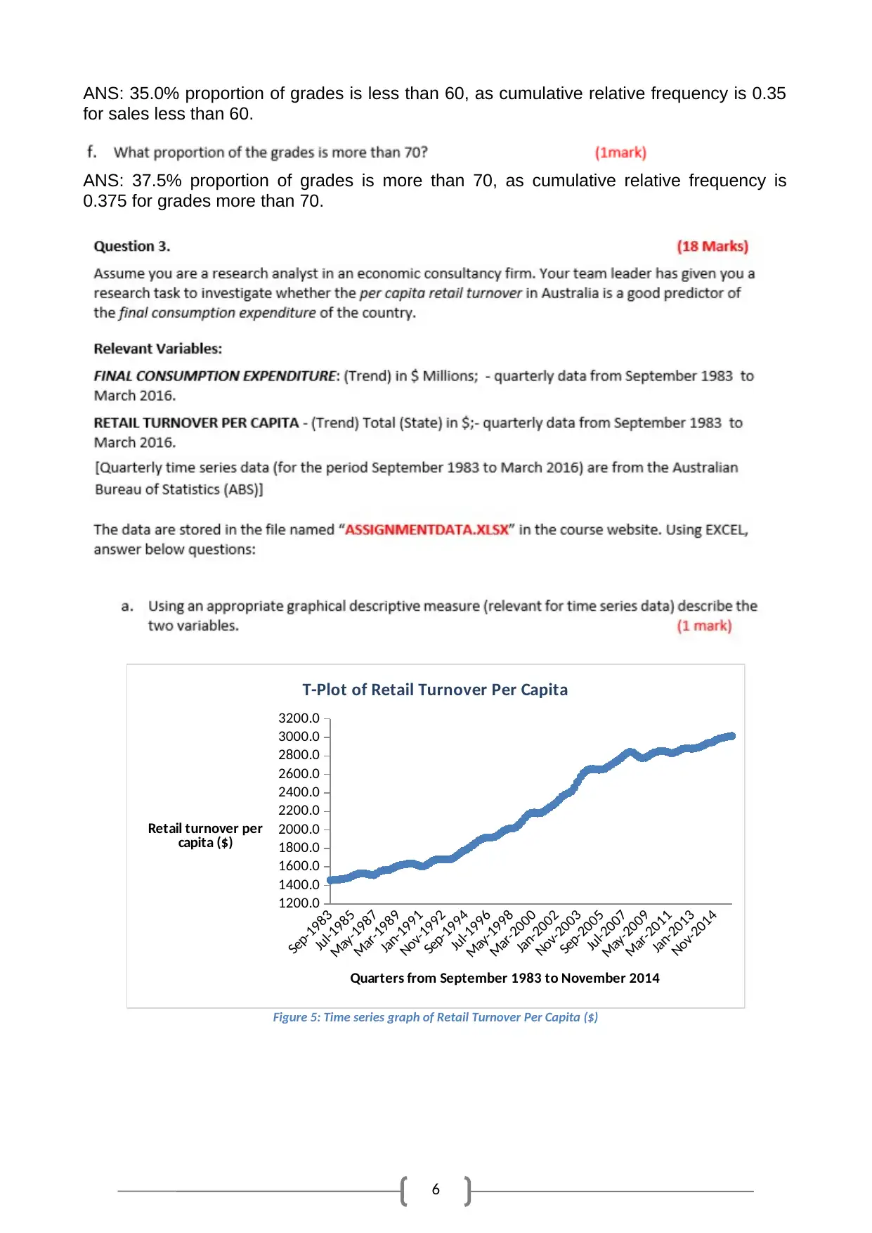
ANS: 35.0% proportion of grades is less than 60, as cumulative relative frequency is 0.35
for sales less than 60.
ANS: 37.5% proportion of grades is more than 70, as cumulative relative frequency is
0.375 for grades more than 70.
Sep-1983
Jul-1985
May-1987
Mar-1989
Jan-1991
Nov-1992
Sep-1994
Jul-1996
May-1998
Mar-2000
Jan-2002
Nov-2003
Sep-2005
Jul-2007
May-2009
Mar-2011
Jan-2013
Nov-2014
1200.0
1400.0
1600.0
1800.0
2000.0
2200.0
2400.0
2600.0
2800.0
3000.0
3200.0
T-Plot of Retail Turnover Per Capita
Quarters from September 1983 to November 2014
Retail turnover per
capita ($)
Figure 5: Time series graph of Retail Turnover Per Capita ($)
7
Sep-1983
Jun-1985
Mar-1987
Dec-1988
Sep-1990
Jun-1992
Mar-1994
Dec-1995
Sep-1997
Jun-1999
Mar-2001
Dec-2002
Sep-2004
Jun-2006
Mar-2008
Dec-2009
Sep-2011
Jun-2013
Mar-2015
57000
77000
97000
117000
137000
157000
177000
197000
217000
237000
257000
T-Plot of Final Consumption Expenditure
Quarters from September 1983 to November 2014
Final Consumption
Expenditure ($
Millions)
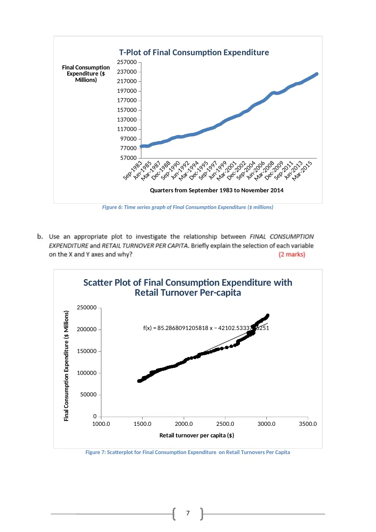
Figure 6: Time series graph of Final Consumption Expenditure ($ millions)
1000.0 1500.0 2000.0 2500.0 3000.0 3500.0
0
50000
100000
150000
200000
250000
f(x) = 85.2868091205818 x − 42102.5333746251
Scatter Plot of Final Consumption Expenditure with
Retail Turnover Per-capita
Retail turnover per capita ($)
Final Consumption Expenditure ($ Millions)
Figure 7: Scatterplot for Final Consumption Expenditure on Retail Turnovers Per Capita
Sep-1983
Jun-1985
Mar-1987
Dec-1988
Sep-1990
Jun-1992
Mar-1994
Dec-1995
Sep-1997
Jun-1999
Mar-2001
Dec-2002
Sep-2004
Jun-2006
Mar-2008
Dec-2009
Sep-2011
Jun-2013
Mar-2015
57000
77000
97000
117000
137000
157000
177000
197000
217000
237000
257000
T-Plot of Final Consumption Expenditure
Quarters from September 1983 to November 2014
Final Consumption
Expenditure ($
Millions)
Figure 6: Time series graph of Final Consumption Expenditure ($ millions)
1000.0 1500.0 2000.0 2500.0 3000.0 3500.0
0
50000
100000
150000
200000
250000
f(x) = 85.2868091205818 x − 42102.5333746251
Scatter Plot of Final Consumption Expenditure with
Retail Turnover Per-capita
Retail turnover per capita ($)
Final Consumption Expenditure ($ Millions)
Figure 7: Scatterplot for Final Consumption Expenditure on Retail Turnovers Per Capita
Paraphrase This Document
Need a fresh take? Get an instant paraphrase of this document with our AI Paraphraser
8
A significant, linear and highly positive correlation is observed between retail turnovers per
capita and final consumption expenditure. Retail Turnovers Per Capita is taken as the
independent variable and taken on X-axis. Final Consumption Expenditure is considered
as the dependent variable and taken on Y axis. Final Consumption Expenditure depends
on individual consumption, and is the income account representing consumer spending.
The choices of X-axis and Y-axis are influenced by this fact.
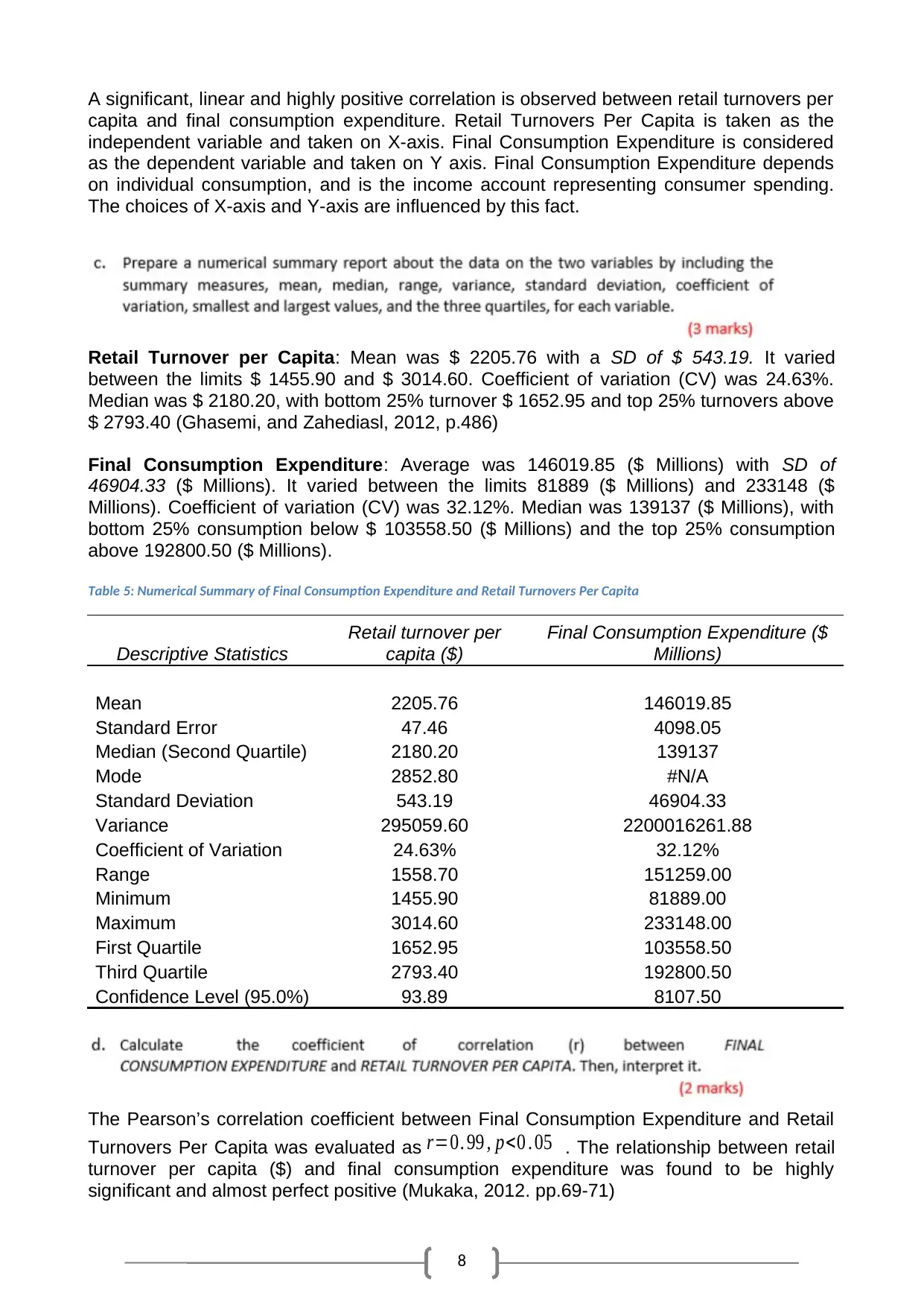
Retail Turnover per Capita: Mean was $ 2205.76 with a SD of $ 543.19. It varied
between the limits $ 1455.90 and $ 3014.60. Coefficient of variation (CV) was 24.63%.
Median was $ 2180.20, with bottom 25% turnover $ 1652.95 and top 25% turnovers above
$ 2793.40 (Ghasemi, and Zahediasl, 2012, p.486)
Final Consumption Expenditure: Average was 146019.85 ($ Millions) with SD of
46904.33 ($ Millions). It varied between the limits 81889 ($ Millions) and 233148 ($
Millions). Coefficient of variation (CV) was 32.12%. Median was 139137 ($ Millions), with
bottom 25% consumption below $ 103558.50 ($ Millions) and the top 25% consumption
above 192800.50 ($ Millions).
Table 5: Numerical Summary of Final Consumption Expenditure and Retail Turnovers Per Capita
Descriptive Statistics
Retail turnover per
capita ($)
Final Consumption Expenditure ($
Millions)
Mean 2205.76 146019.85
Standard Error 47.46 4098.05
Median (Second Quartile) 2180.20 139137
Mode 2852.80 #N/A
Standard Deviation 543.19 46904.33
Variance 295059.60 2200016261.88
Coefficient of Variation 24.63% 32.12%
Range 1558.70 151259.00
Minimum 1455.90 81889.00
Maximum 3014.60 233148.00
First Quartile 1652.95 103558.50
Third Quartile 2793.40 192800.50
Confidence Level (95.0%) 93.89 8107.50
The Pearson’s correlation coefficient between Final Consumption Expenditure and Retail
Turnovers Per Capita was evaluated as r=0. 99 , p<0 . 05 . The relationship between retail
turnover per capita ($) and final consumption expenditure was found to be highly
significant and almost perfect positive (Mukaka, 2012. pp.69-71)
A significant, linear and highly positive correlation is observed between retail turnovers per
capita and final consumption expenditure. Retail Turnovers Per Capita is taken as the
independent variable and taken on X-axis. Final Consumption Expenditure is considered
as the dependent variable and taken on Y axis. Final Consumption Expenditure depends
on individual consumption, and is the income account representing consumer spending.
The choices of X-axis and Y-axis are influenced by this fact.
Retail Turnover per Capita: Mean was $ 2205.76 with a SD of $ 543.19. It varied
between the limits $ 1455.90 and $ 3014.60. Coefficient of variation (CV) was 24.63%.
Median was $ 2180.20, with bottom 25% turnover $ 1652.95 and top 25% turnovers above
$ 2793.40 (Ghasemi, and Zahediasl, 2012, p.486)
Final Consumption Expenditure: Average was 146019.85 ($ Millions) with SD of
46904.33 ($ Millions). It varied between the limits 81889 ($ Millions) and 233148 ($
Millions). Coefficient of variation (CV) was 32.12%. Median was 139137 ($ Millions), with
bottom 25% consumption below $ 103558.50 ($ Millions) and the top 25% consumption
above 192800.50 ($ Millions).
Table 5: Numerical Summary of Final Consumption Expenditure and Retail Turnovers Per Capita
Descriptive Statistics
Retail turnover per
capita ($)
Final Consumption Expenditure ($
Millions)
Mean 2205.76 146019.85
Standard Error 47.46 4098.05
Median (Second Quartile) 2180.20 139137
Mode 2852.80 #N/A
Standard Deviation 543.19 46904.33
Variance 295059.60 2200016261.88
Coefficient of Variation 24.63% 32.12%
Range 1558.70 151259.00
Minimum 1455.90 81889.00
Maximum 3014.60 233148.00
First Quartile 1652.95 103558.50
Third Quartile 2793.40 192800.50
Confidence Level (95.0%) 93.89 8107.50
The Pearson’s correlation coefficient between Final Consumption Expenditure and Retail
Turnovers Per Capita was evaluated as r=0. 99 , p<0 . 05 . The relationship between retail
turnover per capita ($) and final consumption expenditure was found to be highly
significant and almost perfect positive (Mukaka, 2012. pp.69-71)
9
.
Table 6: Regression Summary of Final Consumption Expenditure on Retail Turnovers Per Capita
Regression Statistics
Multiple R 0.99
R Square 0.98
Adjusted R Square 0.98
Standard Error 7363.23
Observations 131
ANOVA
df SS MS F
Significance
F
Regression 1 279008109980.07 279008109980.07 5146.13 0.0000
Residual 129 6994004064.18 54217085.77
Total 130 286002114044.24
Regression Coefficients Standard
Error t Stat P-
value
Lower
95%
Upper
95%
Intercept -42102.53 2700.17 -
15.59 0.000 -47444.88 -36760.19
Retail turnover per capita
($) 85.29 1.19 71.74 0.000 82.93 87.64
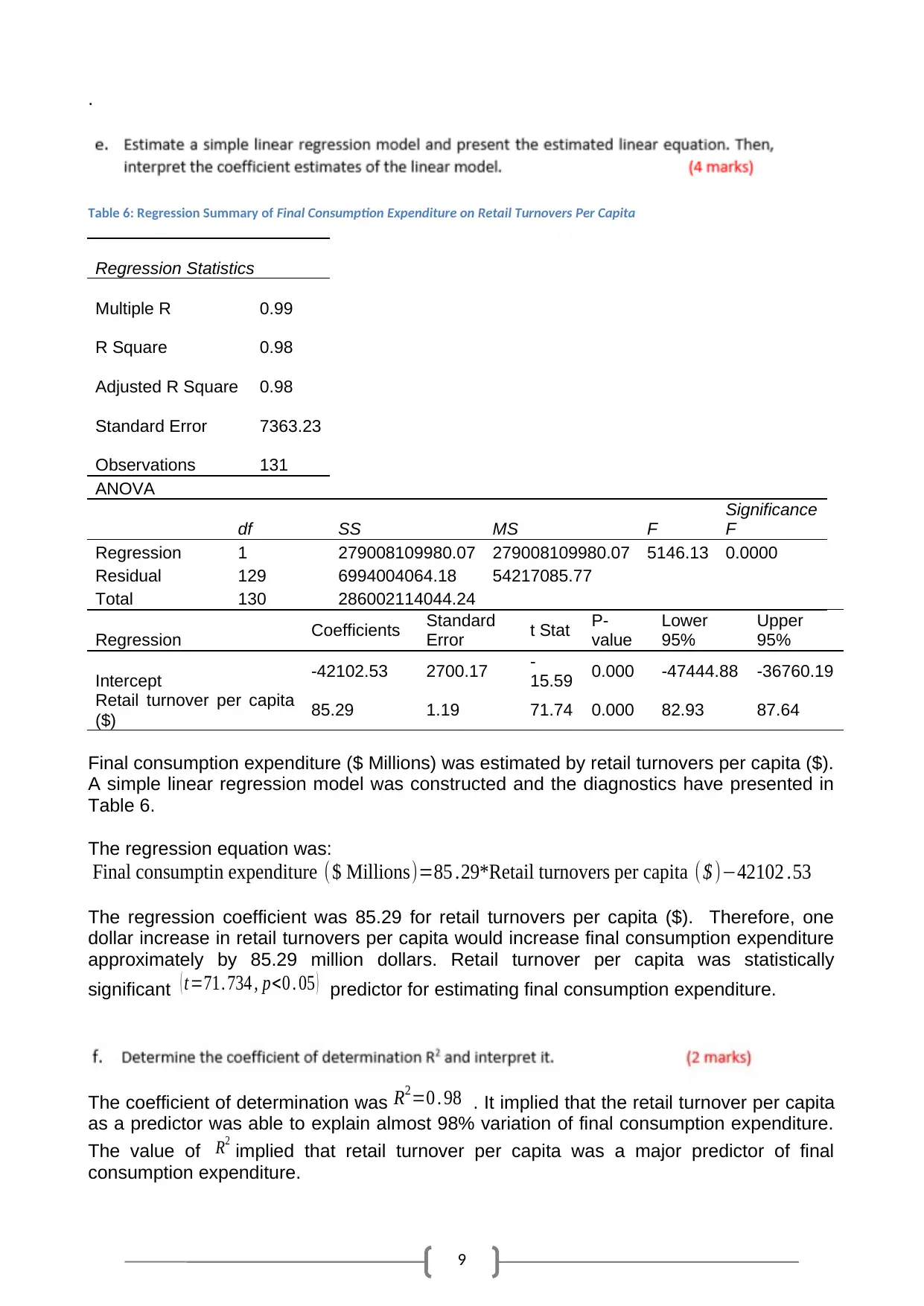
Final consumption expenditure ($ Millions) was estimated by retail turnovers per capita ($).
A simple linear regression model was constructed and the diagnostics have presented in
Table 6.
The regression equation was:
Final consumptin expenditure ($ Millions)=85 .29*Retail turnovers per capita ( $ )−42102 .53
The regression coefficient was 85.29 for retail turnovers per capita ($). Therefore, one
dollar increase in retail turnovers per capita would increase final consumption expenditure
approximately by 85.29 million dollars. Retail turnover per capita was statistically
significant ( t=71. 734 , p<0 . 05 ) predictor for estimating final consumption expenditure.
The coefficient of determination was R2=0 . 98 . It implied that the retail turnover per capita
as a predictor was able to explain almost 98% variation of final consumption expenditure.
The value of R2
implied that retail turnover per capita was a major predictor of final
consumption expenditure.
.
Table 6: Regression Summary of Final Consumption Expenditure on Retail Turnovers Per Capita
Regression Statistics
Multiple R 0.99
R Square 0.98
Adjusted R Square 0.98
Standard Error 7363.23
Observations 131
ANOVA
df SS MS F
Significance
F
Regression 1 279008109980.07 279008109980.07 5146.13 0.0000
Residual 129 6994004064.18 54217085.77
Total 130 286002114044.24
Regression Coefficients Standard
Error t Stat P-
value
Lower
95%
Upper
95%
Intercept -42102.53 2700.17 -
15.59 0.000 -47444.88 -36760.19
Retail turnover per capita
($) 85.29 1.19 71.74 0.000 82.93 87.64
Final consumption expenditure ($ Millions) was estimated by retail turnovers per capita ($).
A simple linear regression model was constructed and the diagnostics have presented in
Table 6.
The regression equation was:
Final consumptin expenditure ($ Millions)=85 .29*Retail turnovers per capita ( $ )−42102 .53
The regression coefficient was 85.29 for retail turnovers per capita ($). Therefore, one
dollar increase in retail turnovers per capita would increase final consumption expenditure
approximately by 85.29 million dollars. Retail turnover per capita was statistically
significant ( t=71. 734 , p<0 . 05 ) predictor for estimating final consumption expenditure.
The coefficient of determination was R2=0 . 98 . It implied that the retail turnover per capita
as a predictor was able to explain almost 98% variation of final consumption expenditure.
The value of R2
implied that retail turnover per capita was a major predictor of final
consumption expenditure.
10
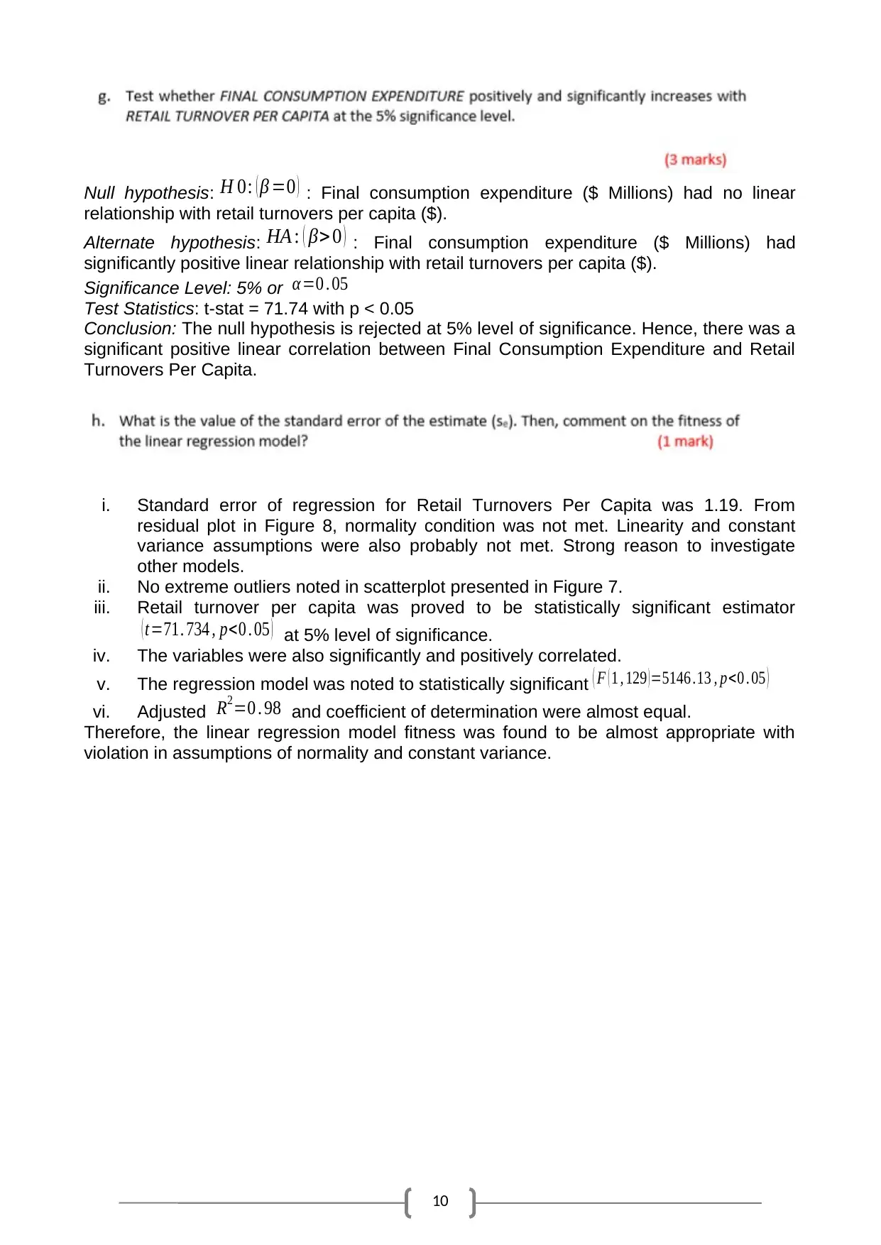
Null hypothesis: H 0: ( β =0 ) : Final consumption expenditure ($ Millions) had no linear
relationship with retail turnovers per capita ($).
Alternate hypothesis: HA : ( β> 0 ) : Final consumption expenditure ($ Millions) had
significantly positive linear relationship with retail turnovers per capita ($).
Significance Level: 5% or α=0 . 05
Test Statistics: t-stat = 71.74 with p < 0.05
Conclusion: The null hypothesis is rejected at 5% level of significance. Hence, there was a
significant positive linear correlation between Final Consumption Expenditure and Retail
Turnovers Per Capita.
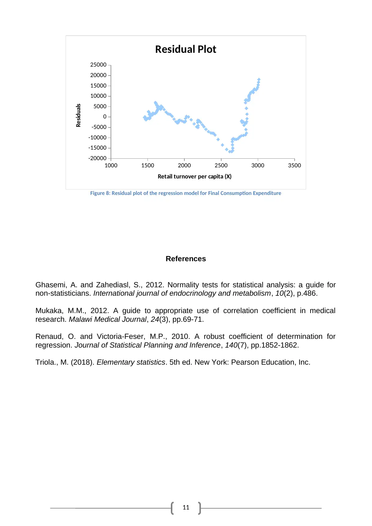
i. Standard error of regression for Retail Turnovers Per Capita was 1.19. From
residual plot in Figure 8, normality condition was not met. Linearity and constant
variance assumptions were also probably not met. Strong reason to investigate
other models.
ii. No extreme outliers noted in scatterplot presented in Figure 7.
iii. Retail turnover per capita was proved to be statistically significant estimator
( t=71. 734 , p<0 . 05 ) at 5% level of significance.
iv. The variables were also significantly and positively correlated.
v. The regression model was noted to statistically significant ( F ( 1 , 129 ) =5146 .13 , p<0 . 05 )
vi. Adjusted R2=0 . 98 and coefficient of determination were almost equal.
Therefore, the linear regression model fitness was found to be almost appropriate with
violation in assumptions of normality and constant variance.
Null hypothesis: H 0: ( β =0 ) : Final consumption expenditure ($ Millions) had no linear
relationship with retail turnovers per capita ($).
Alternate hypothesis: HA : ( β> 0 ) : Final consumption expenditure ($ Millions) had
significantly positive linear relationship with retail turnovers per capita ($).
Significance Level: 5% or α=0 . 05
Test Statistics: t-stat = 71.74 with p < 0.05
Conclusion: The null hypothesis is rejected at 5% level of significance. Hence, there was a
significant positive linear correlation between Final Consumption Expenditure and Retail
Turnovers Per Capita.
i. Standard error of regression for Retail Turnovers Per Capita was 1.19. From
residual plot in Figure 8, normality condition was not met. Linearity and constant
variance assumptions were also probably not met. Strong reason to investigate
other models.
ii. No extreme outliers noted in scatterplot presented in Figure 7.
iii. Retail turnover per capita was proved to be statistically significant estimator
( t=71. 734 , p<0 . 05 ) at 5% level of significance.
iv. The variables were also significantly and positively correlated.
v. The regression model was noted to statistically significant ( F ( 1 , 129 ) =5146 .13 , p<0 . 05 )
vi. Adjusted R2=0 . 98 and coefficient of determination were almost equal.
Therefore, the linear regression model fitness was found to be almost appropriate with
violation in assumptions of normality and constant variance.
Secure Best Marks with AI Grader
Need help grading? Try our AI Grader for instant feedback on your assignments.
11
1000 1500 2000 2500 3000 3500
-20000
-15000
-10000
-5000
0
5000
10000
15000
20000
25000
Residual Plot
Retail turnover per capita (X)
Residuals
Figure 8: Residual plot of the regression model for Final Consumption Expenditure
References
Ghasemi, A. and Zahediasl, S., 2012. Normality tests for statistical analysis: a guide for
non-statisticians. International journal of endocrinology and metabolism, 10(2), p.486.
Mukaka, M.M., 2012. A guide to appropriate use of correlation coefficient in medical
research. Malawi Medical Journal, 24(3), pp.69-71.
Renaud, O. and Victoria-Feser, M.P., 2010. A robust coefficient of determination for
regression. Journal of Statistical Planning and Inference, 140(7), pp.1852-1862.
Triola., M. (2018). Elementary statistics. 5th ed. New York: Pearson Education, Inc.
1 out of 11
Related Documents


Your All-in-One AI-Powered Toolkit for Academic Success.
+13062052269
info@desklib.com
Available 24*7 on WhatsApp / Email
![[object Object]](/_next/static/media/star-bottom.7253800d.svg)
Unlock your academic potential
© 2024 | Zucol Services PVT LTD | All rights reserved.