Business Statistics Assignment 2
VerifiedAdded on 2023/06/11
|34
|6311
|80
AI Summary
This article contains solutions to Business Statistics Assignment 2. It includes questions related to confidence intervals, hypothesis testing, and sample size calculations. The subject is Business Statistics.
Contribute Materials
Your contribution can guide someone’s learning journey. Share your
documents today.

Running head: BUSINESS STATISTICS
Business Statistics
Assignment 2
Name of the Student:
Name of the University:
Author Note:
Business Statistics
Assignment 2
Name of the Student:
Name of the University:
Author Note:
Secure Best Marks with AI Grader
Need help grading? Try our AI Grader for instant feedback on your assignments.
1BUSINESS STATISTICS
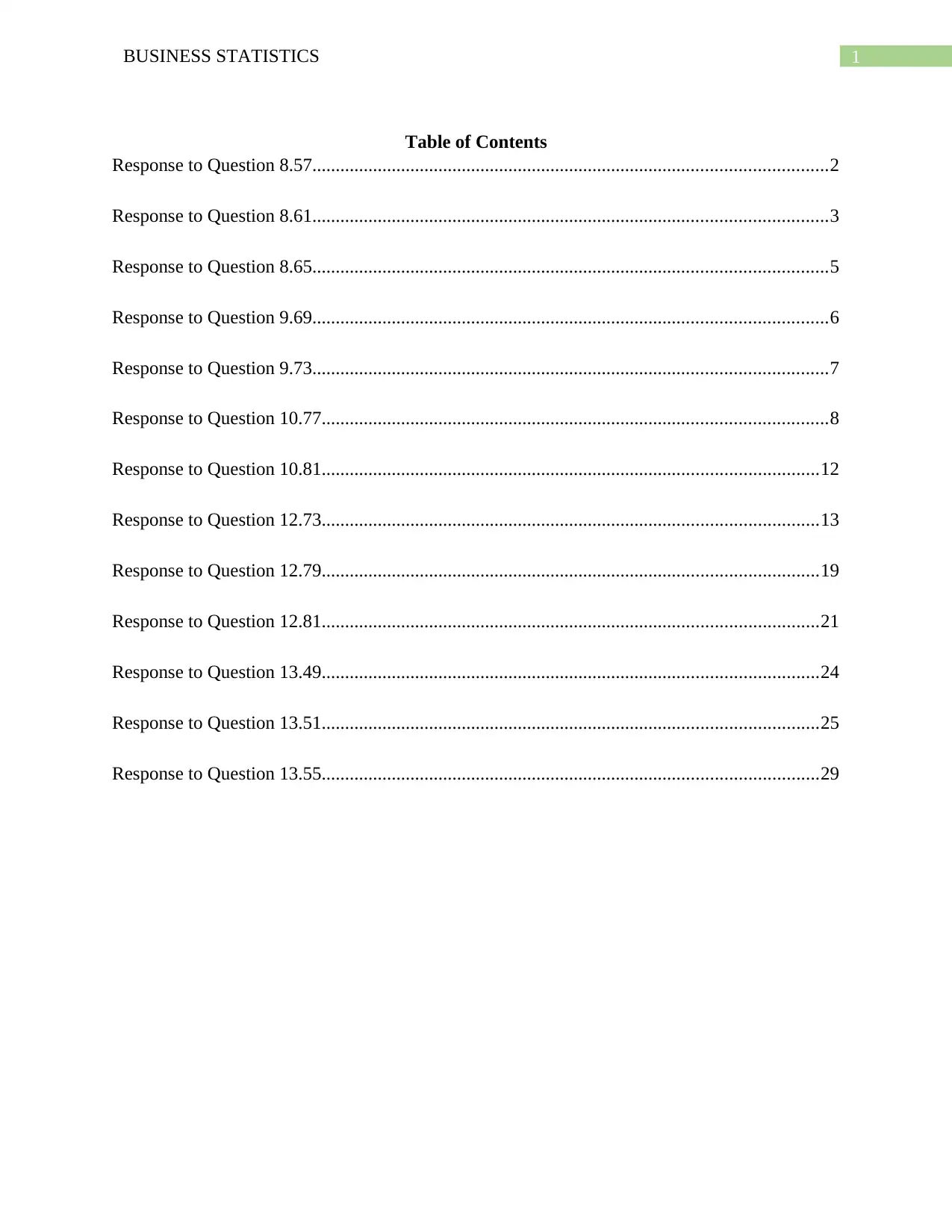
Table of Contents
Response to Question 8.57..............................................................................................................2
Response to Question 8.61..............................................................................................................3
Response to Question 8.65..............................................................................................................5
Response to Question 9.69..............................................................................................................6
Response to Question 9.73..............................................................................................................7
Response to Question 10.77............................................................................................................8
Response to Question 10.81..........................................................................................................12
Response to Question 12.73..........................................................................................................13
Response to Question 12.79..........................................................................................................19
Response to Question 12.81..........................................................................................................21
Response to Question 13.49..........................................................................................................24
Response to Question 13.51..........................................................................................................25
Response to Question 13.55..........................................................................................................29
2BUSINESS STATISTICS
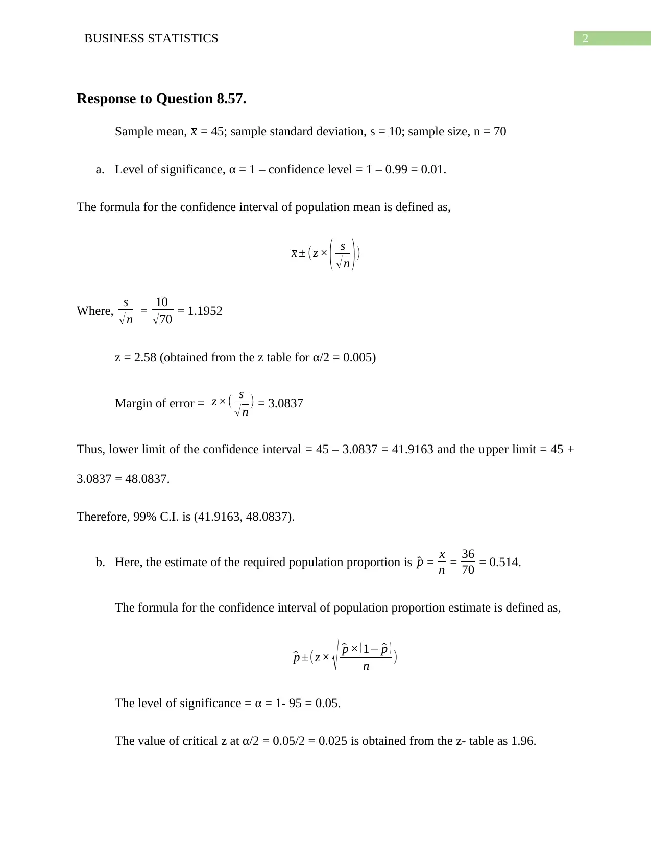
Response to Question 8.57.
Sample mean, x = 45; sample standard deviation, s = 10; sample size, n = 70
a. Level of significance, α = 1 – confidence level = 1 – 0.99 = 0.01.
The formula for the confidence interval of population mean is defined as,
x ± (z × ( s
√ n ) )
Where, s
√n = 10
√ 70 = 1.1952
z = 2.58 (obtained from the z table for α/2 = 0.005)
Margin of error = z ×( s
√ n ) = 3.0837
Thus, lower limit of the confidence interval = 45 – 3.0837 = 41.9163 and the upper limit = 45 +
3.0837 = 48.0837.
Therefore, 99% C.I. is (41.9163, 48.0837).
b. Here, the estimate of the required population proportion is ^p = x
n = 36
70 = 0.514.
The formula for the confidence interval of population proportion estimate is defined as,
^p ±(z × √ ^p × ( 1− ^p )
n )
The level of significance = α = 1- 95 = 0.05.
The value of critical z at α/2 = 0.05/2 = 0.025 is obtained from the z- table as 1.96.
3BUSINESS STATISTICS
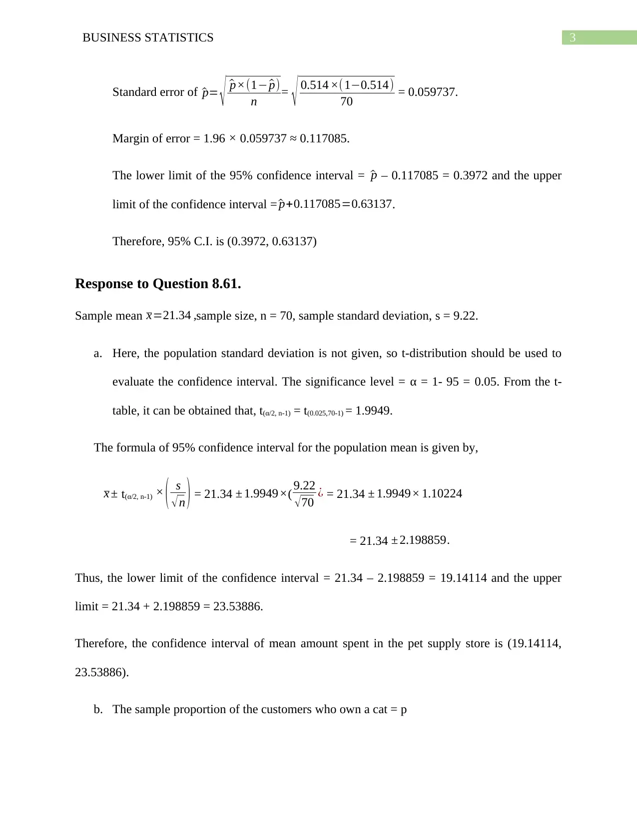
Standard error of ^p= √ ^p×(1− ^p)
n = √ 0.514 ×( 1−0.514)
70 = 0.059737.
Margin of error = 1.96 × 0.059737 ≈ 0.117085.
The lower limit of the 95% confidence interval = ^p – 0.117085 = 0.3972 and the upper
limit of the confidence interval = ^p+0.117085=0.63137.
Therefore, 95% C.I. is (0.3972, 0.63137)
Response to Question 8.61.
Sample mean x=21.34 ,sample size, n = 70, sample standard deviation, s = 9.22.
a. Here, the population standard deviation is not given, so t-distribution should be used to
evaluate the confidence interval. The significance level = α = 1- 95 = 0.05. From the t-
table, it can be obtained that, t(α/2, n-1) = t(0.025,70-1) = 1.9949.
The formula of 95% confidence interval for the population mean is given by,
x ± t(α/2, n-1) × ( s
√ n ) = 21.34 ± 1.9949×( 9.22
√ 70 ¿ = 21.34 ± 1.9949× 1.10224
= 21.34 ± 2.198859.
Thus, the lower limit of the confidence interval = 21.34 – 2.198859 = 19.14114 and the upper
limit = 21.34 + 2.198859 = 23.53886.
Therefore, the confidence interval of mean amount spent in the pet supply store is (19.14114,
23.53886).
b. The sample proportion of the customers who own a cat = p
Secure Best Marks with AI Grader
Need help grading? Try our AI Grader for instant feedback on your assignments.
4BUSINESS STATISTICS
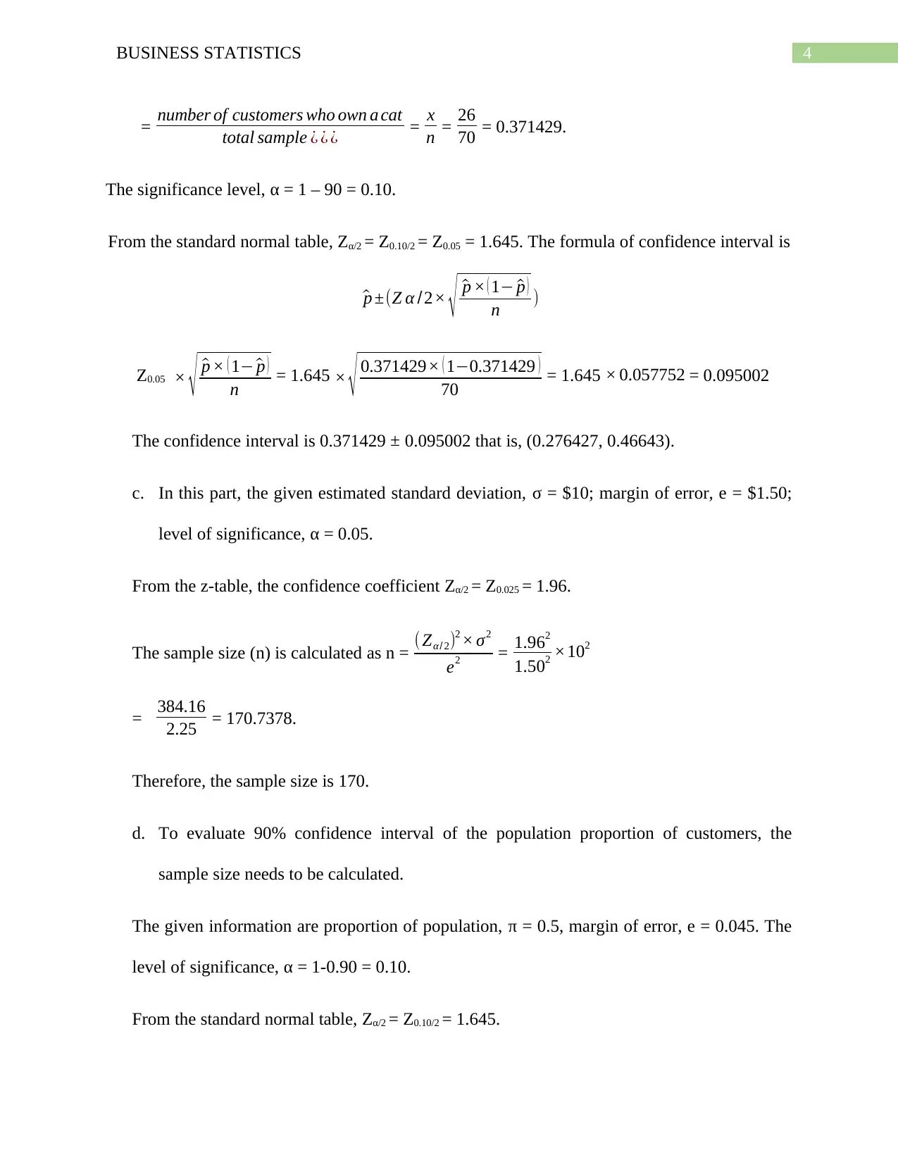
= number of customers who own a cat
total sample ¿ ¿ ¿ = x
n = 26
70 = 0.371429.
The significance level, α = 1 – 90 = 0.10.
From the standard normal table, Zα/2 = Z0.10/2 = Z0.05 = 1.645. The formula of confidence interval is
^p ±(Z α /2× √ ^p × ( 1− ^p )
n )
Z0.05 × √ ^p × ( 1− ^p )
n = 1.645 × √ 0.371429× ( 1−0.371429 )
70 = 1.645 × 0.057752 = 0.095002
The confidence interval is 0.371429 ± 0.095002 that is, (0.276427, 0.46643).
c. In this part, the given estimated standard deviation, σ = $10; margin of error, e = $1.50;
level of significance, α = 0.05.
From the z-table, the confidence coefficient Zα/2 = Z0.025 = 1.96.
The sample size (n) is calculated as n = ( Zα/ 2)2 × σ2
e2 = 1.962
1.502 ×102
= 384.16
2.25 = 170.7378.
Therefore, the sample size is 170.
d. To evaluate 90% confidence interval of the population proportion of customers, the
sample size needs to be calculated.
The given information are proportion of population, π = 0.5, margin of error, e = 0.045. The
level of significance, α = 1-0.90 = 0.10.
From the standard normal table, Zα/2 = Z0.10/2 = 1.645.
5BUSINESS STATISTICS
Thus, the required sample size, n = ( Zα/ 2)2 × π ×(1−π )
e2 = 1.6452
0.0452 ×0.5 ×(1−0.5) =
0.676506
0.002025 = 334.0772.
Therefore, the sample size is 335.
e. From the calculated sample sizes in (c) and (d), the manager should take the sample size
of 335 as the sample size is larger in the latter case.
Response to Question 8.65.
The given information are sample mean, x = 5.5, standard deviation, s = 0.099, sample size, n =
50. The standard error, e = s/√ n = 0.099/50 = 0.014.
a. At 99% confidence level, the level of significance, α = 1-0.99 = 0.01.
The critical value of z at α = 0.01 is 2.58 (from the z-table).
The confidence interval is given by x ±2.58× 0.014.
The margin of error = 2.58 × 0.014 = 0.0362.
Therefore, the 99% confidence interval for the population mean weight is given by 5.5 ± 0.0362
that is, (5.4638,5.5362).
b. The problem requires to perform a t-test to check whether the mean amount of tea in the
bag is 5.5 grams or not. Thus, the null hypothesis is H0: μ = 5.5 against the alternative
hypothesis H1: μ≠ 5.5.
The sample mean is calculated from the given data of 50 observation and it is 5.497.
6BUSINESS STATISTICS
It is clearly seen that the sample mean lies within the confidence interval. Thus, the null
hypothesis is accepted and it can be concluded that the company is meeting the requirement
of containing 5.5 grams tea in the tea bag.
c. Yes, the assumptions are valid to calculate the 99% confidence interval.
Response to Question 9.69.
a. The null and the alternative hypotheses are stated respectively as,
H0: The proportion of population of web page visitors preferring the new design is 0.50.
H1: The proportion of population of web page visitors preferring the new design is not 0.50
b. The type I error occurs if the null hypothesis, being true, is rejected by the investigator.
The type II error occurs when the false null hypothesis is accepted by the investigator.
In the given course of problem, when the population proportion of web page visitors
preferring the new design is truly 0.50 but the investigator reject the null hypothesis, then
type I error occurs. Again, if the investigator accepts the null hypothesis when the
population proportion of web page visitors preferring the new design is actually not 0.50,
then the type II error occurs.
c. At 5% level of significance, the p-value of 0.20 is greater than α = 0.05. Thus, the null
hypothesis is accepted here as there is not enough evidence to state that the null
hypothesis is wrong. Therefore, the population proportion is 0.50. If the null hypothesis is
rejected here then the type I error will occur.
d. If the value of α is raised, then the possibility of rejecting the null hypothesis will be
increased. Thus, it will actually help to increase the probability of accepting H0.
Paraphrase This Document
Need a fresh take? Get an instant paraphrase of this document with our AI Paraphraser
7BUSINESS STATISTICS
e. The sample size can also be increased instead of increasing the level of significance,
which will help to represent the population in better way. The larger the sample size, the
better will be the representation of the population.
f. If the p-value is 0.12, then also the level of significance will be less than p-value which
will again lead to accept the null hypothesis.
If the p-value is reduced to 0.06, then also the null hypothesis will not be rejected as the
p-value is still greater than the significance level.
Response to Question 9.73.
a. The sample standard deviation is √ 34.552
75 = 3.99.
The null hypothesis for the required test is given by
H0: μ ≥ 100 against the alternative hypothesis H1: μ < 100 where μ denotes the population
mean.
The test statistic, tcal = (
93.70−100
34.55
√ 75
) = -1.58 with degrees of freedom 75-1 = 74 and the
significance level = 0.05
The critical value of t-statistic is -1.6657 which is greater than 0.05. Thus, the null
hypothesis is accepted and there is not enough evidence to state that the mean
reimbursement is less than $100.
b. The requires test of hypotheses are
H0: π ≤ 0.10 against H1: π > 0.10; where π is the population proportion.
8BUSINESS STATISTICS
Sample proportion p = 12/75 = 0.16
The calculated value of the test-statistic of this one-tail z-test =
0.16−0.10
√ (0.10)(1−0.10)
75
= 1.73.
The null hypothesis is rejected as 1.73> 1.64, where 1.64 is the critical z-value at 5% level of
significance.
c. The assumption behind the t-test is that the sample is drawn from normally distributed
population.
d. If the sample mean is $90 then the revised value of test statistic = (
90−100
34.55
√ 75
) = -2.51.
Clearly, -2.51< -1.64, the null hypothesis is rejected at 5% level of significance and the mean
reimbursement value will be less than $100.
e. For 15 office visits the modified value of proportion = 15/75 = 0.20.
The revised z-statistic value =
0.20−0.10
√ ( 0.10)( 1−0.10)
75
= 2.89.
At 5% significance level, the H0 will be rejected here as 2.89>1.64. Thus, there is enough
proof to have the population proportion more than 0.10.
Response to Question 10.77.
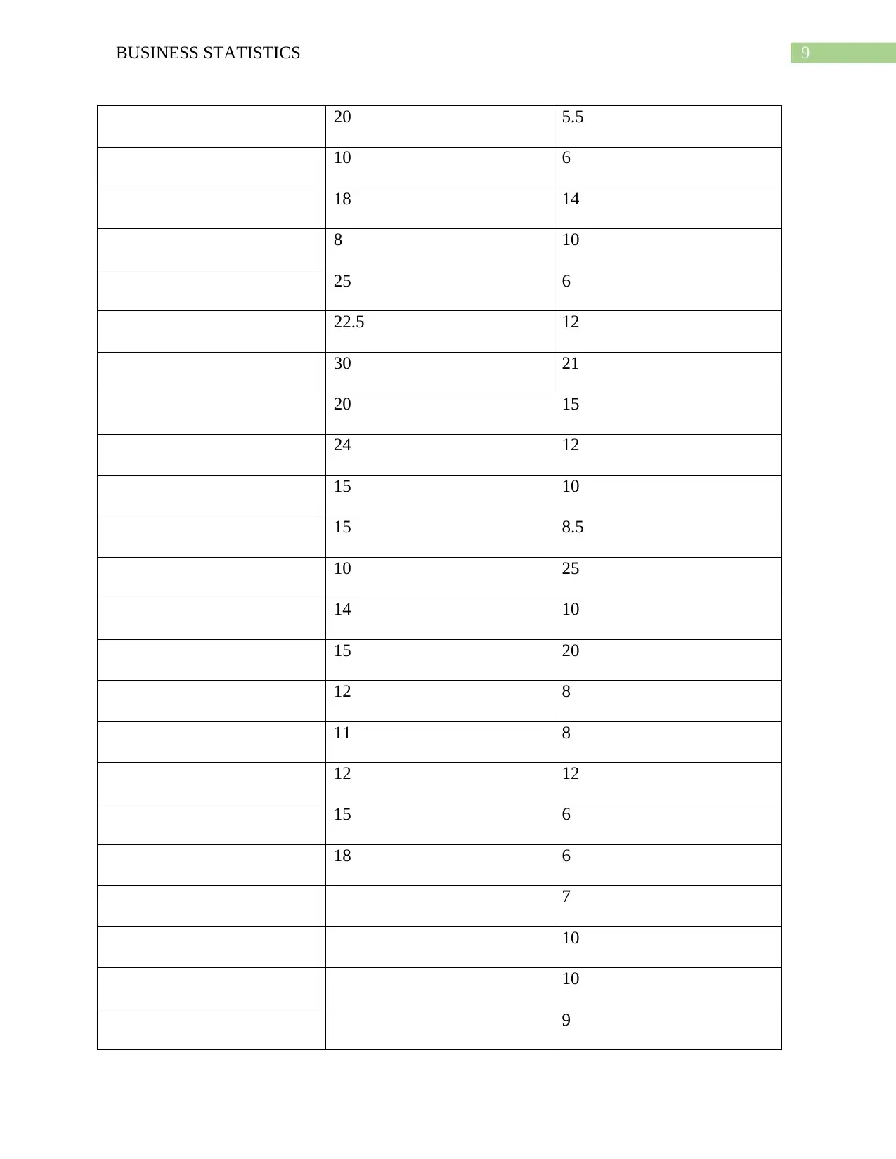
The required calculations are shown in the following table
Measurements Gender (Female) Gender (Male)
18 10
9BUSINESS STATISTICS
20 5.5
10 6
18 14
8 10
25 6
22.5 12
30 21
20 15
24 12
15 10
15 8.5
10 25
14 10
15 20
12 8
11 8
12 12
15 6
18 6
7
10
10
9
20 5.5
10 6
18 14
8 10
25 6
22.5 12
30 21
20 15
24 12
15 10
15 8.5
10 25
14 10
15 20
12 8
11 8
12 12
15 6
18 6
7
10
10
9
Secure Best Marks with AI Grader
Need help grading? Try our AI Grader for instant feedback on your assignments.
10BUSINESS STATISTICS
10
30
10
10
5
5
10
11
15
15
7
8
12
10
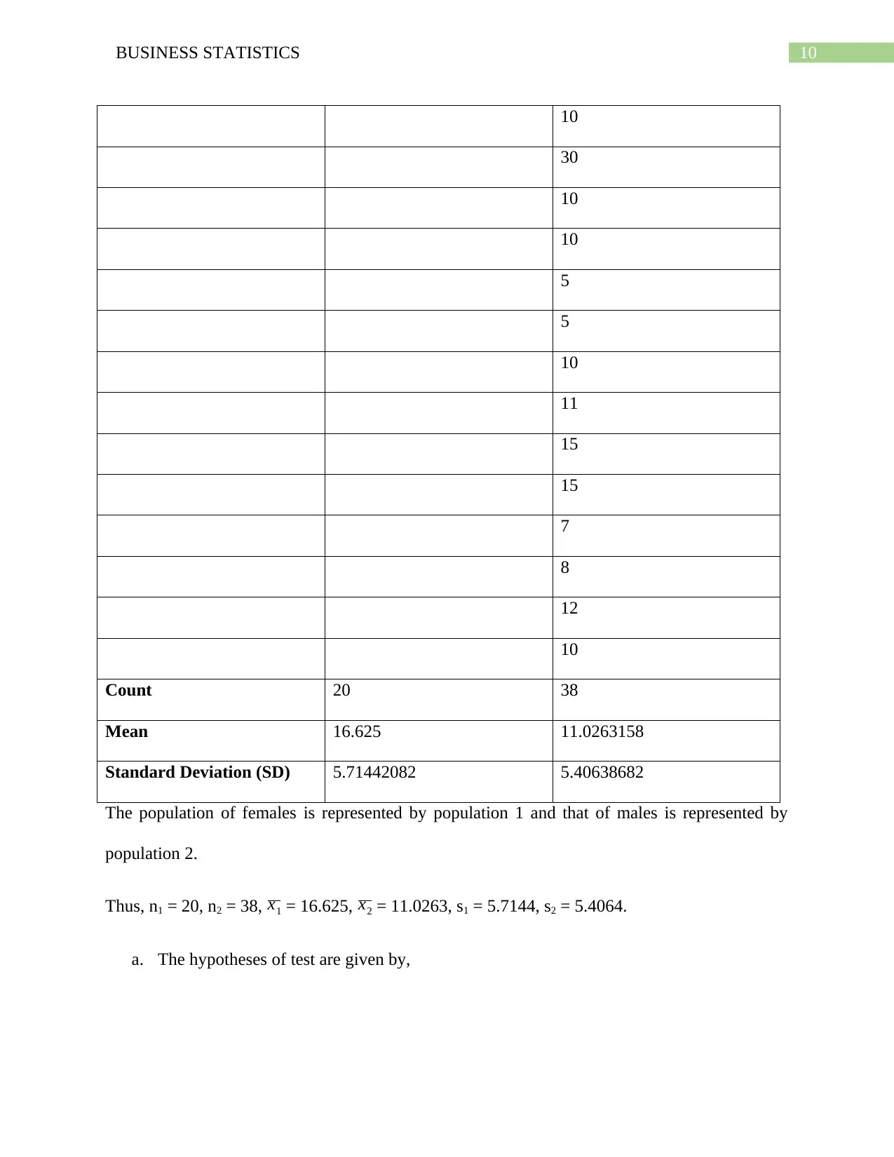
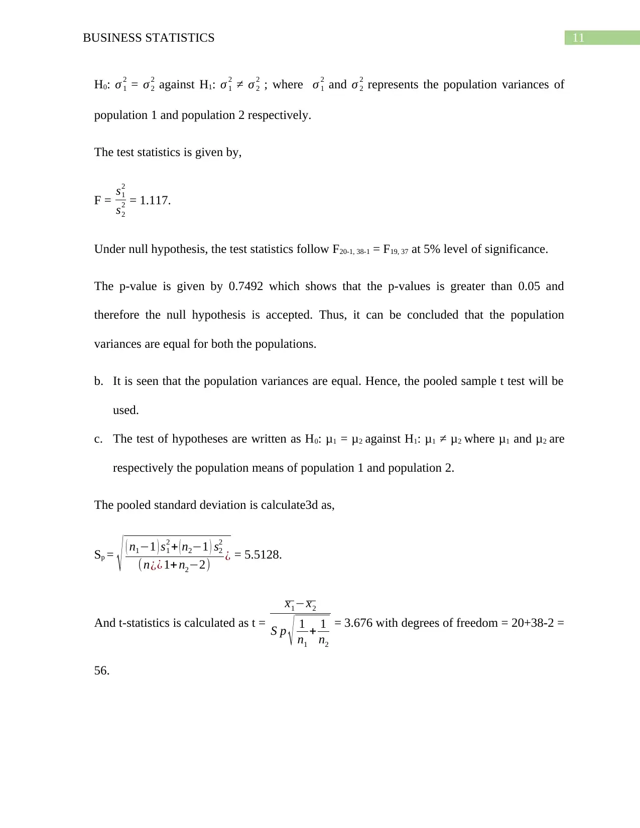
Count 20 38
Mean 16.625 11.0263158
Standard Deviation (SD) 5.71442082 5.40638682
The population of females is represented by population 1 and that of males is represented by
population 2.
Thus, n1 = 20, n2 = 38, x1 = 16.625, x2 = 11.0263, s1 = 5.7144, s2 = 5.4064.
a. The hypotheses of test are given by,
10
30
10
10
5
5
10
11
15
15
7
8
12
10
Count 20 38
Mean 16.625 11.0263158
Standard Deviation (SD) 5.71442082 5.40638682
The population of females is represented by population 1 and that of males is represented by
population 2.
Thus, n1 = 20, n2 = 38, x1 = 16.625, x2 = 11.0263, s1 = 5.7144, s2 = 5.4064.
a. The hypotheses of test are given by,
11BUSINESS STATISTICS
H0: σ 1
2 = σ 2
2 against H1: σ 1
2 ≠ σ 2
2 ; where σ 1
2 and σ 2
2 represents the population variances of
population 1 and population 2 respectively.
The test statistics is given by,
F = s1
2
s2
2 = 1.117.
Under null hypothesis, the test statistics follow F20-1, 38-1 = F19, 37 at 5% level of significance.
The p-value is given by 0.7492 which shows that the p-values is greater than 0.05 and
therefore the null hypothesis is accepted. Thus, it can be concluded that the population
variances are equal for both the populations.
b. It is seen that the population variances are equal. Hence, the pooled sample t test will be
used.
c. The test of hypotheses are written as H0: μ1 = μ2 against H1: μ1 ≠ μ2 where μ1 and μ2 are
respectively the population means of population 1 and population 2.
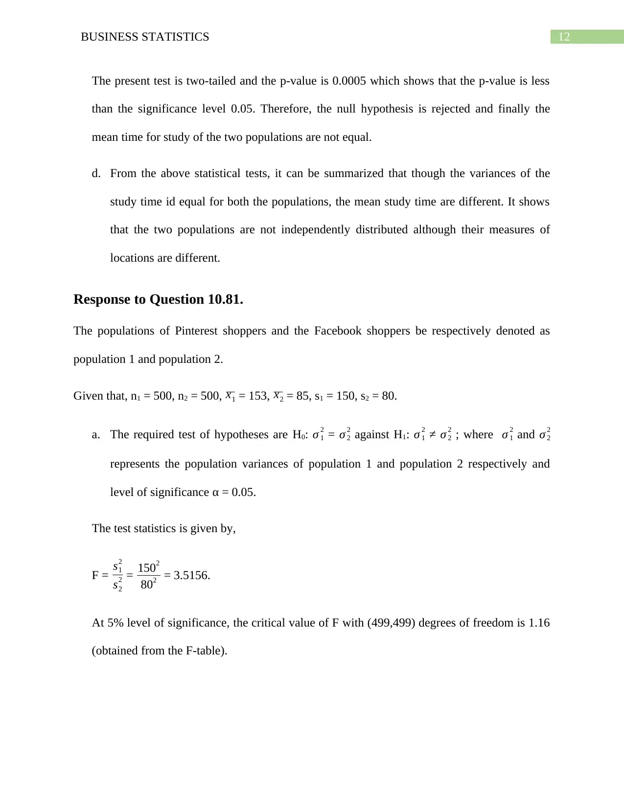
The pooled standard deviation is calculate3d as,
Sp =
√ ( n1−1 ) s1
2 + ( n2−1 ) s2
2
(n¿¿ 1+ n2−2) ¿ = 5.5128.
And t-statistics is calculated as t =
x1−x2
S p √ 1
n1
+ 1
n2
= 3.676 with degrees of freedom = 20+38-2 =
56.
12BUSINESS STATISTICS
The present test is two-tailed and the p-value is 0.0005 which shows that the p-value is less
than the significance level 0.05. Therefore, the null hypothesis is rejected and finally the
mean time for study of the two populations are not equal.
d. From the above statistical tests, it can be summarized that though the variances of the
study time id equal for both the populations, the mean study time are different. It shows
that the two populations are not independently distributed although their measures of
locations are different.
Response to Question 10.81.
The populations of Pinterest shoppers and the Facebook shoppers be respectively denoted as
population 1 and population 2.
Given that, n1 = 500, n2 = 500, x1 = 153, x2 = 85, s1 = 150, s2 = 80.
a. The required test of hypotheses are H0: σ 1
2 = σ 2
2 against H1: σ 1
2 ≠ σ 2
2 ; where σ 1
2 and σ 2
2
represents the population variances of population 1 and population 2 respectively and
level of significance α = 0.05.
The test statistics is given by,
F = s1
2
s2
2 = 1502
802 = 3.5156.
At 5% level of significance, the critical value of F with (499,499) degrees of freedom is 1.16
(obtained from the F-table).
Paraphrase This Document
Need a fresh take? Get an instant paraphrase of this document with our AI Paraphraser
13BUSINESS STATISTICS
Thus, the observed value of F is greater than the critical value of F which leads to reject the
null hypothesis. Therefore there is difference in the variance of the order values of Pinterest
shoppers and the Facebook shoppers.
b. The test of hypotheses are H0: μ1 = μ2 against H1: μ1 ≠ μ2 where μ1 and μ2 are respectively
the population means of population 1 and population 2.
The pooled variance is S2 = ( n1−1 ) s1
2 + ( n2−1 ) s2
2
(n¿ ¿1+ n2−2)¿ = 12526.15
The test statistic is t =
x1−x2
S p √ 1
n1
+ 1
n2
= 9.61.
The critical value of t statistic with df = 500+500-2 = 998 at 5% level of significance is given
as 1.96.
The critical value is less than the calculated value of t-statistic. Thus, the null hypothesis is
rejected and finally the mean time for study of the two populations are not equal.
c. The 95% confidence interval for the difference of mean values is obtained by the
following calculation
μ1 - μ2 = x1 - x2 ± tα/ 2 √ s1
2
n1
+ s2
2
n2
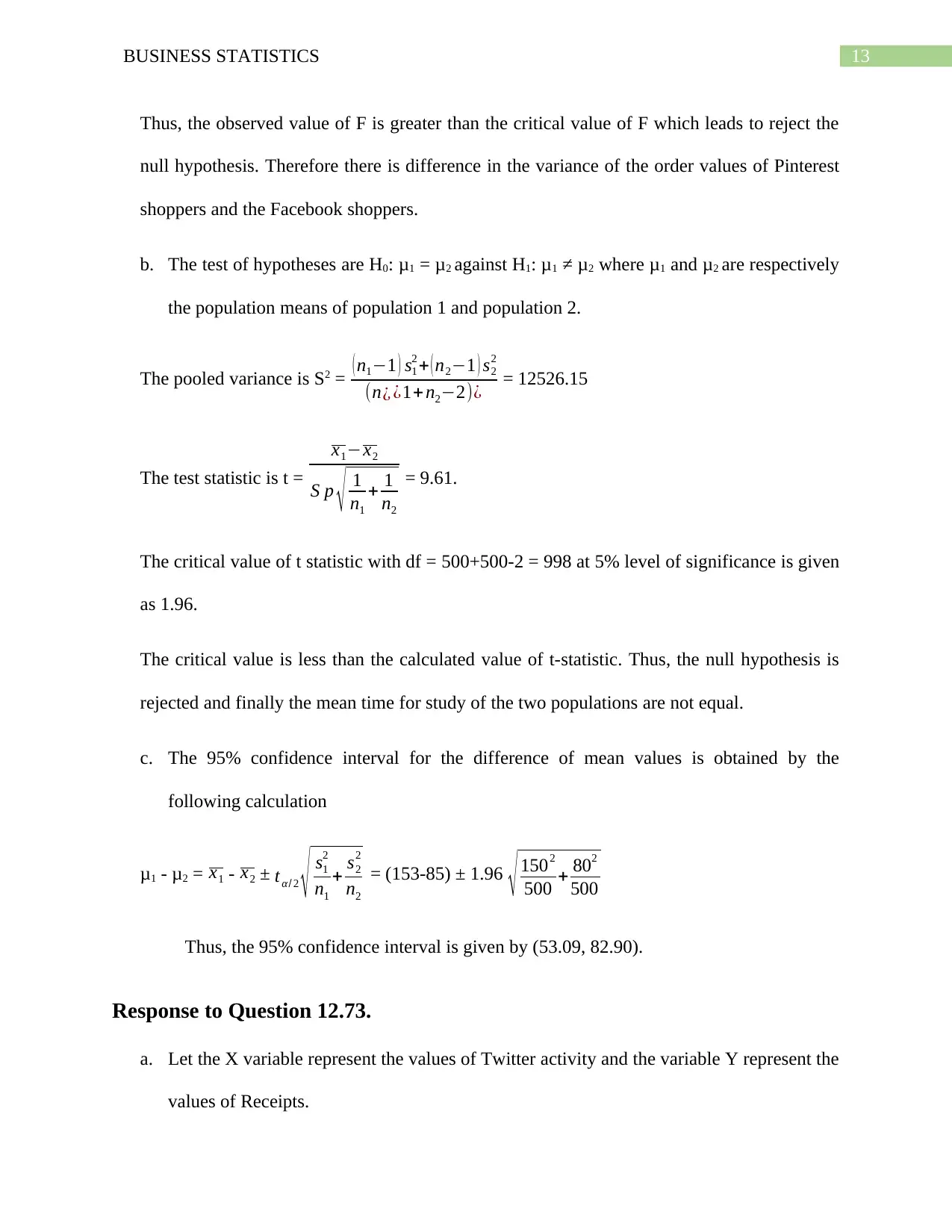
= (153-85) ± 1.96 √ 1502
500 + 802
500
Thus, the 95% confidence interval is given by (53.09, 82.90).
Response to Question 12.73.
a. Let the X variable represent the values of Twitter activity and the variable Y represent the
values of Receipts.
14BUSINESS STATISTICS
Therefore, the simple linear regression equation is given by:
^Y i=b0 +b1 Xi
Where ^Y iis the estimated value of Y corresponding to the values of X, b0 is the y-intercept of
the sample and b1 is the sample slope. The values of i run from 1 to 7.
The Data Analysis Tool Pak of MS Excel is used to calculate the simple linear regression
line.
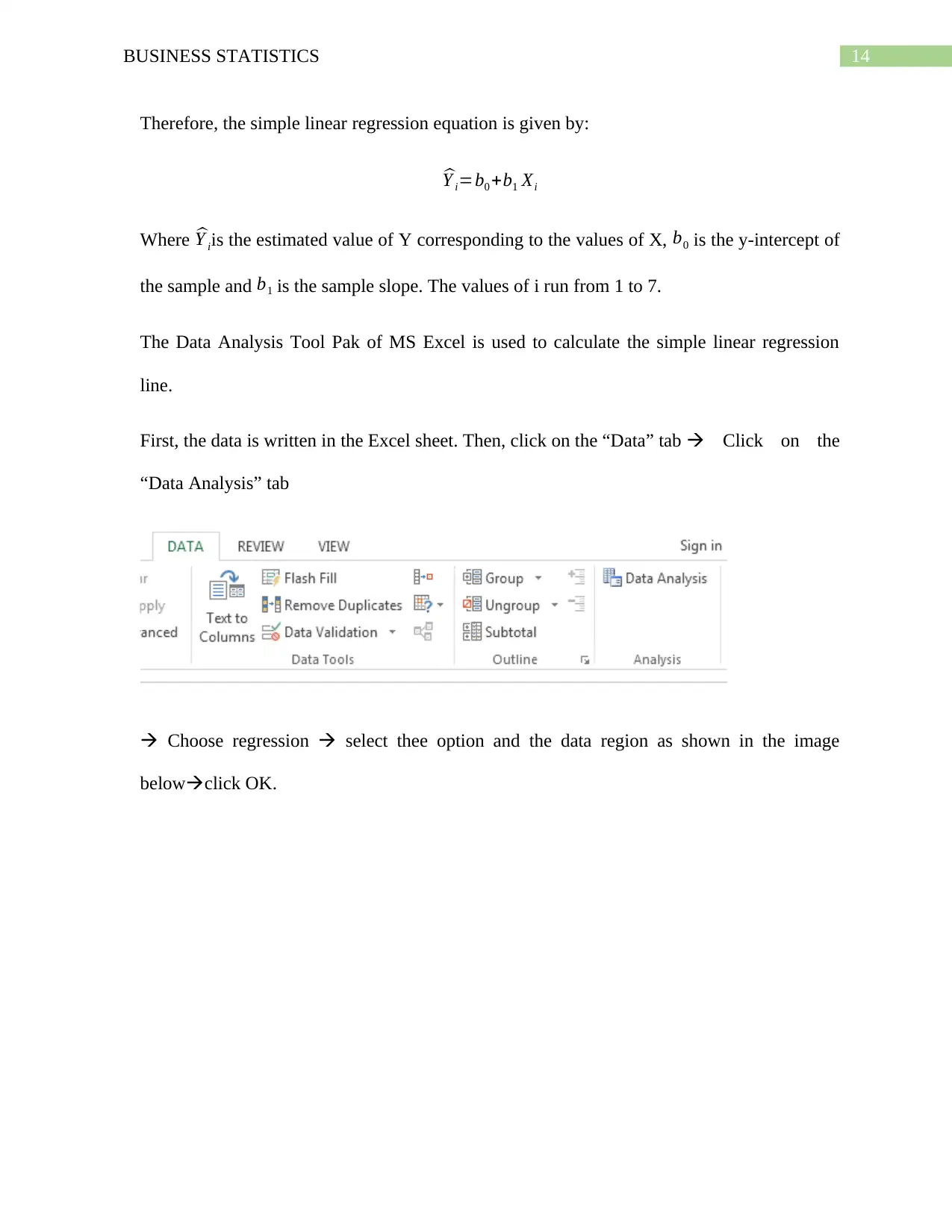
First, the data is written in the Excel sheet. Then, click on the “Data” tab Click on the
“Data Analysis” tab
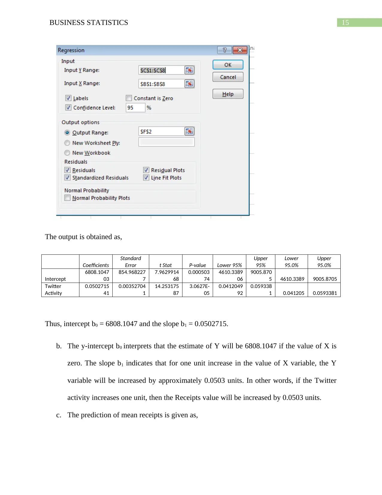
Choose regression select thee option and the data region as shown in the image
belowclick OK.
15BUSINESS STATISTICS
The output is obtained as,
Coefficients
Standard
Error t Stat P-value Lower 95%
Upper
95%
Lower
95.0%
Upper
95.0%
Intercept
6808.1047
03
854.968227
7
7.9629914
68
0.000503
74
4610.3389
06
9005.870
5 4610.3389 9005.8705
Twitter
Activity
0.0502715
41
0.00352704
1
14.253175
87
3.0627E-
05
0.0412049
92
0.059338
1 0.041205 0.0593381
Thus, intercept b0 = 6808.1047 and the slope b1 = 0.0502715.
b. The y-intercept b0 interprets that the estimate of Y will be 6808.1047 if the value of X is
zero. The slope b1 indicates that for one unit increase in the value of X variable, the Y
variable will be increased by approximately 0.0503 units. In other words, if the Twitter
activity increases one unit, then the Receipts value will be increased by 0.0503 units.
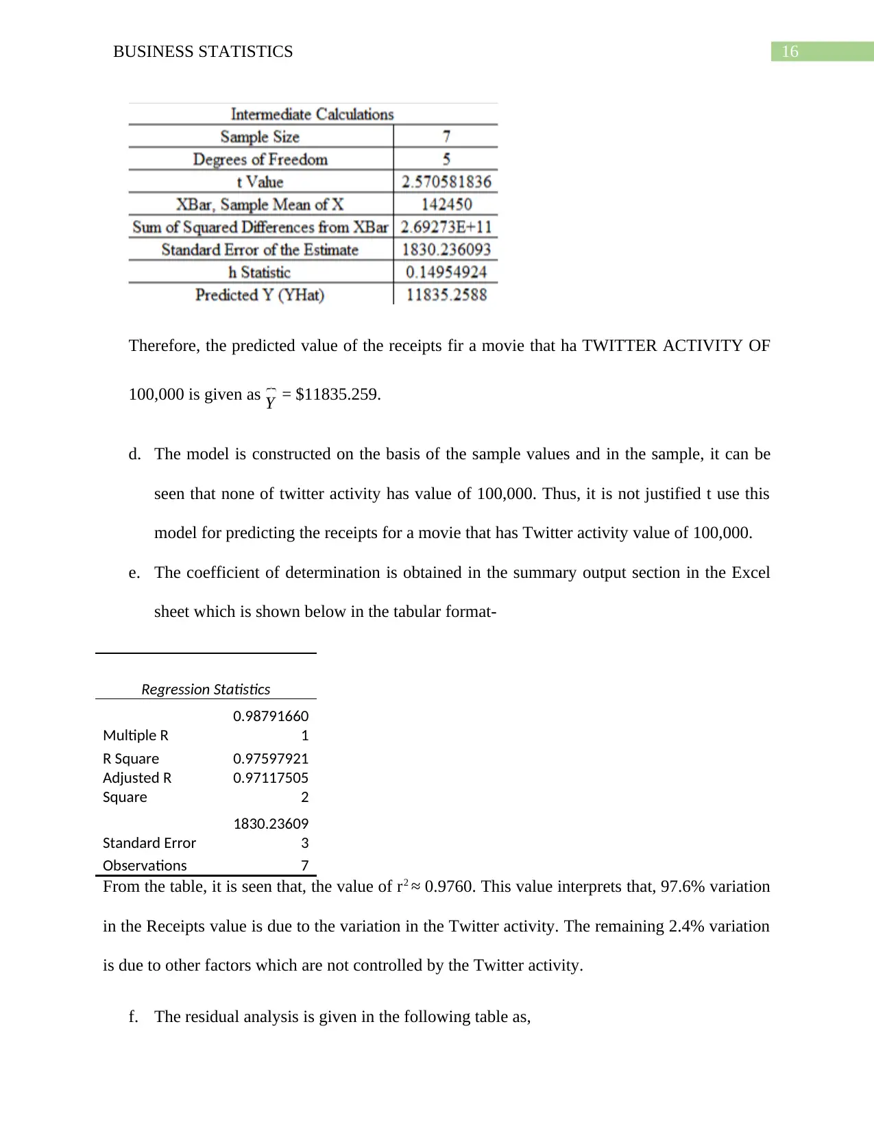
c. The prediction of mean receipts is given as,
The output is obtained as,
Coefficients
Standard
Error t Stat P-value Lower 95%
Upper
95%
Lower
95.0%
Upper
95.0%
Intercept
6808.1047
03
854.968227
7
7.9629914
68
0.000503
74
4610.3389
06
9005.870
5 4610.3389 9005.8705
Activity
0.0502715
41
0.00352704
1
14.253175
87
3.0627E-
05
0.0412049
92
0.059338
1 0.041205 0.0593381
Thus, intercept b0 = 6808.1047 and the slope b1 = 0.0502715.
b. The y-intercept b0 interprets that the estimate of Y will be 6808.1047 if the value of X is
zero. The slope b1 indicates that for one unit increase in the value of X variable, the Y
variable will be increased by approximately 0.0503 units. In other words, if the Twitter
activity increases one unit, then the Receipts value will be increased by 0.0503 units.
c. The prediction of mean receipts is given as,
Secure Best Marks with AI Grader
Need help grading? Try our AI Grader for instant feedback on your assignments.
16BUSINESS STATISTICS
Therefore, the predicted value of the receipts fir a movie that ha TWITTER ACTIVITY OF
100,000 is given as Y⏞ = $11835.259.
d. The model is constructed on the basis of the sample values and in the sample, it can be
seen that none of twitter activity has value of 100,000. Thus, it is not justified t use this
model for predicting the receipts for a movie that has Twitter activity value of 100,000.
e. The coefficient of determination is obtained in the summary output section in the Excel
sheet which is shown below in the tabular format-
Regression Statistics
Multiple R
0.98791660
1
R Square 0.97597921
Adjusted R
Square
0.97117505
2
Standard Error
1830.23609
3
Observations 7
From the table, it is seen that, the value of r2 ≈ 0.9760. This value interprets that, 97.6% variation
in the Receipts value is due to the variation in the Twitter activity. The remaining 2.4% variation
is due to other factors which are not controlled by the Twitter activity.
f. The residual analysis is given in the following table as,
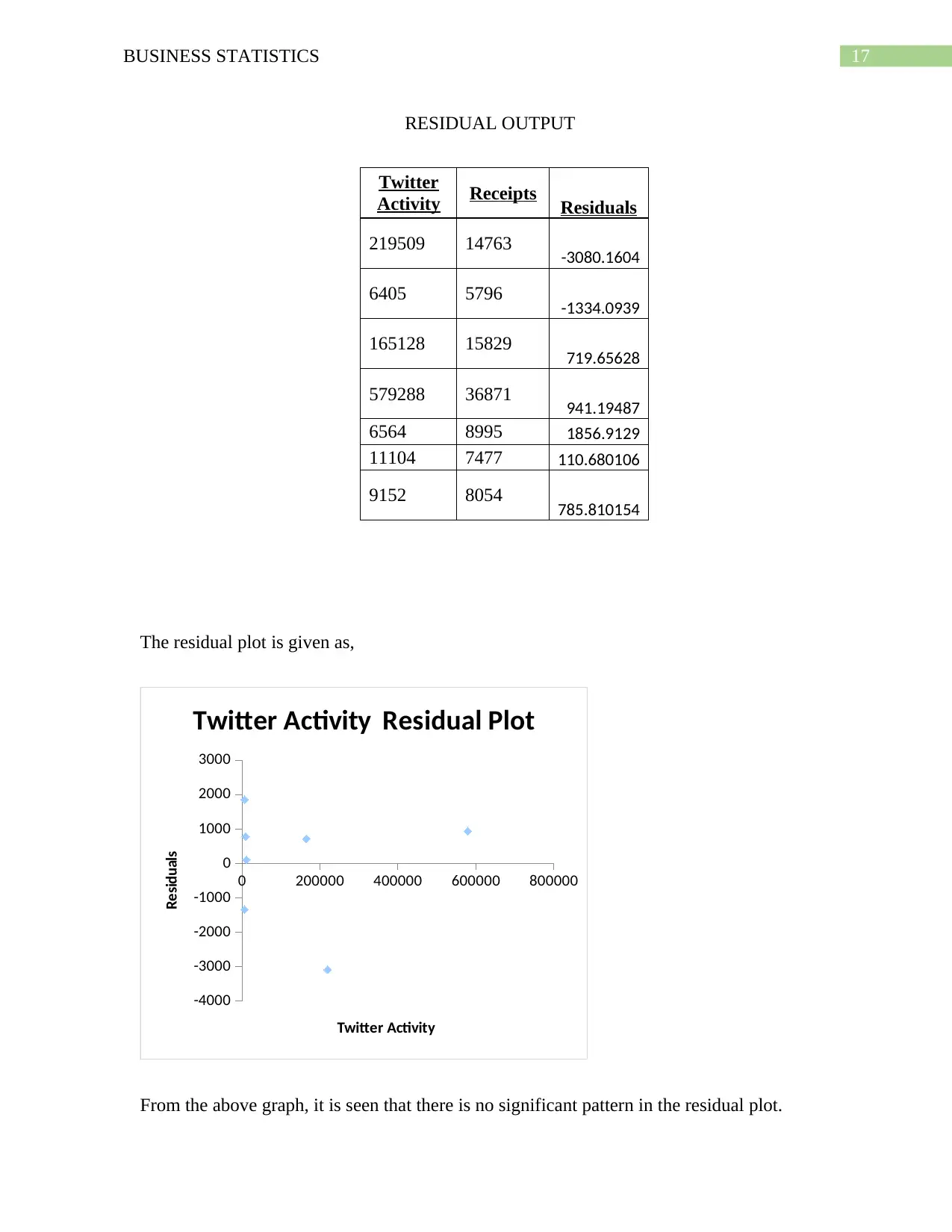
17BUSINESS STATISTICS
RESIDUAL OUTPUT
Twitter
Activity Receipts Residuals
219509 14763 -3080.1604
6405 5796 -1334.0939
165128 15829 719.65628
579288 36871 941.19487
6564 8995 1856.9129
11104 7477 110.680106
9152 8054 785.810154
The residual plot is given as,
0 200000 400000 600000 800000
-4000
-3000
-2000
-1000
0
1000
2000
3000
Twitter Activity Residual Plot
Twitter Activity
Residuals
From the above graph, it is seen that there is no significant pattern in the residual plot.
RESIDUAL OUTPUT
Activity Receipts Residuals
219509 14763 -3080.1604
6405 5796 -1334.0939
165128 15829 719.65628
579288 36871 941.19487
6564 8995 1856.9129
11104 7477 110.680106
9152 8054 785.810154
The residual plot is given as,
0 200000 400000 600000 800000
-4000
-3000
-2000
-1000
0
1000
2000
3000
Twitter Activity Residual Plot
Twitter Activity
Residuals
From the above graph, it is seen that there is no significant pattern in the residual plot.
18BUSINESS STATISTICS
g. To check whether there is any evidence of linear relationship between the two variables
or not, the t-test is performed. The null and the alternative hypotheses are as follows:
H0: β1 = 0 (There is no linear relationship)
H1: β1≠ 0 (There is a linear relationship)
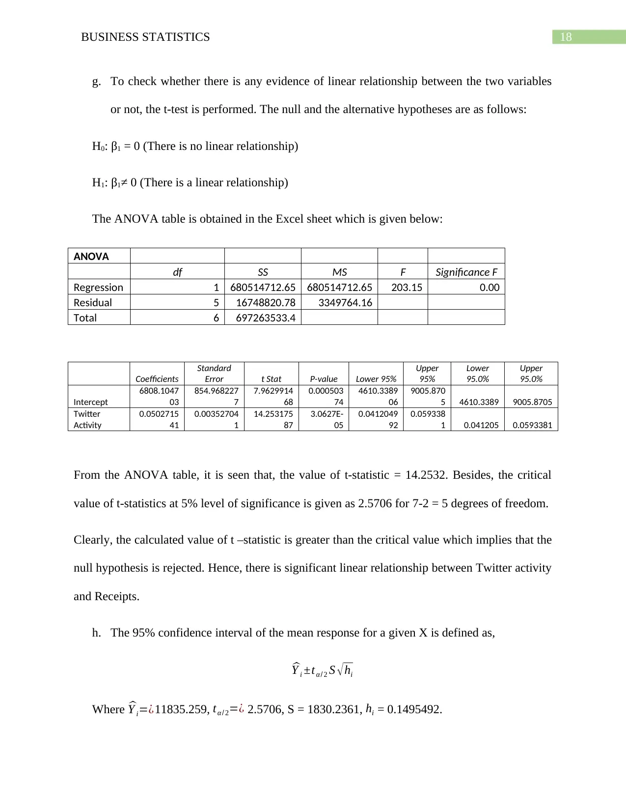
The ANOVA table is obtained in the Excel sheet which is given below:
ANOVA
df SS MS F Significance F
Regression 1 680514712.65 680514712.65 203.15 0.00
Residual 5 16748820.78 3349764.16
Total 6 697263533.4
Coefficients
Standard
Error t Stat P-value Lower 95%
Upper
95%
Lower
95.0%
Upper
95.0%
Intercept
6808.1047
03
854.968227
7
7.9629914
68
0.000503
74
4610.3389
06
9005.870
5 4610.3389 9005.8705
Twitter
Activity
0.0502715
41
0.00352704
1
14.253175
87
3.0627E-
05
0.0412049
92
0.059338
1 0.041205 0.0593381
From the ANOVA table, it is seen that, the value of t-statistic = 14.2532. Besides, the critical
value of t-statistics at 5% level of significance is given as 2.5706 for 7-2 = 5 degrees of freedom.
Clearly, the calculated value of t –statistic is greater than the critical value which implies that the
null hypothesis is rejected. Hence, there is significant linear relationship between Twitter activity
and Receipts.
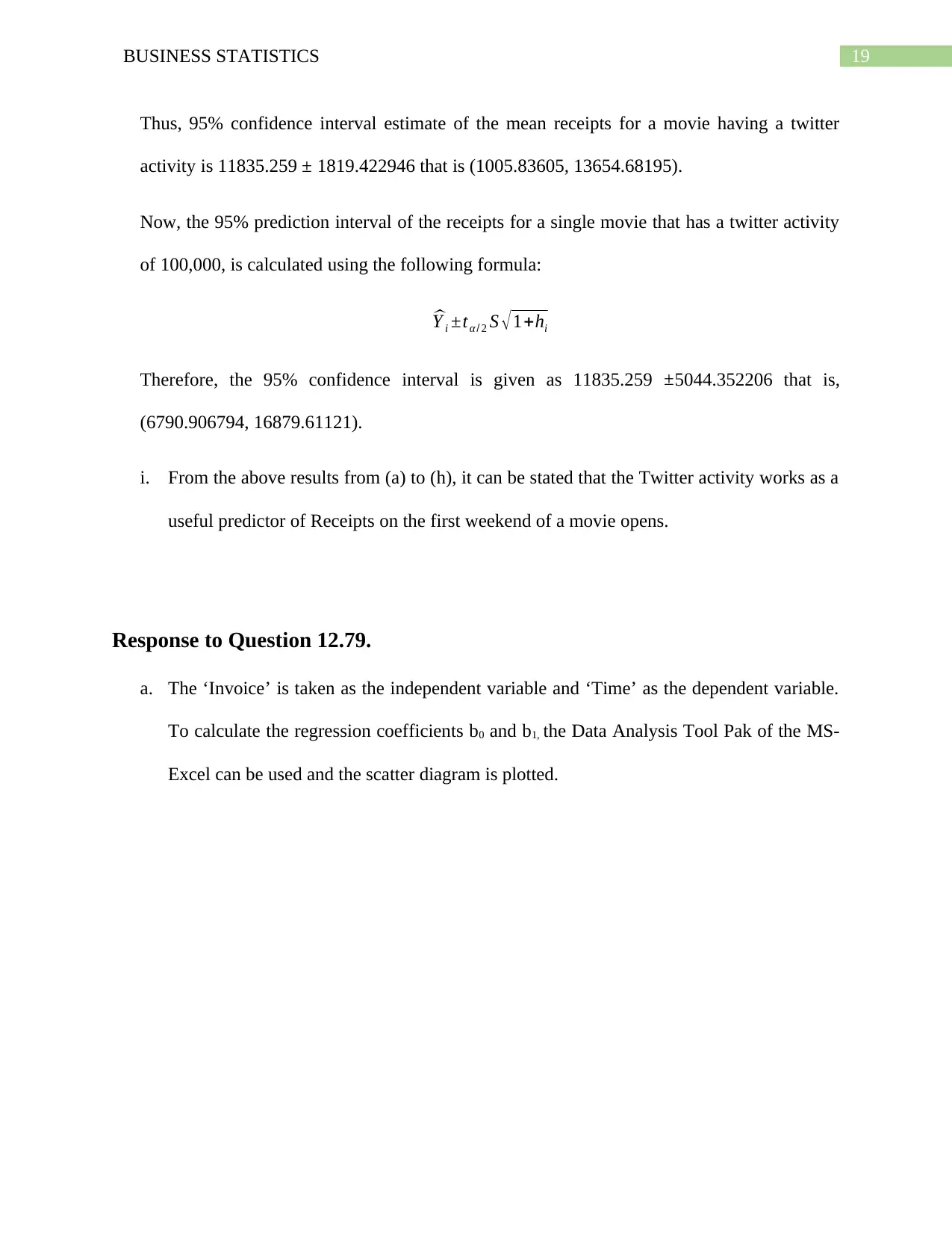
h. The 95% confidence interval of the mean response for a given X is defined as,
^Y i ±tα / 2 S √ hi
Where ^Y i=¿11835.259, tα / 2=¿ 2.5706, S = 1830.2361, hi = 0.1495492.
g. To check whether there is any evidence of linear relationship between the two variables
or not, the t-test is performed. The null and the alternative hypotheses are as follows:
H0: β1 = 0 (There is no linear relationship)
H1: β1≠ 0 (There is a linear relationship)
The ANOVA table is obtained in the Excel sheet which is given below:
ANOVA
df SS MS F Significance F
Regression 1 680514712.65 680514712.65 203.15 0.00
Residual 5 16748820.78 3349764.16
Total 6 697263533.4
Coefficients
Standard
Error t Stat P-value Lower 95%
Upper
95%
Lower
95.0%
Upper
95.0%
Intercept
6808.1047
03
854.968227
7
7.9629914
68
0.000503
74
4610.3389
06
9005.870
5 4610.3389 9005.8705
Activity
0.0502715
41
0.00352704
1
14.253175
87
3.0627E-
05
0.0412049
92
0.059338
1 0.041205 0.0593381
From the ANOVA table, it is seen that, the value of t-statistic = 14.2532. Besides, the critical
value of t-statistics at 5% level of significance is given as 2.5706 for 7-2 = 5 degrees of freedom.
Clearly, the calculated value of t –statistic is greater than the critical value which implies that the
null hypothesis is rejected. Hence, there is significant linear relationship between Twitter activity
and Receipts.
h. The 95% confidence interval of the mean response for a given X is defined as,
^Y i ±tα / 2 S √ hi
Where ^Y i=¿11835.259, tα / 2=¿ 2.5706, S = 1830.2361, hi = 0.1495492.
Paraphrase This Document
Need a fresh take? Get an instant paraphrase of this document with our AI Paraphraser
19BUSINESS STATISTICS
Thus, 95% confidence interval estimate of the mean receipts for a movie having a twitter
activity is 11835.259 ± 1819.422946 that is (1005.83605, 13654.68195).
Now, the 95% prediction interval of the receipts for a single movie that has a twitter activity
of 100,000, is calculated using the following formula:
^Y i ±tα / 2 S √ 1+hi
Therefore, the 95% confidence interval is given as 11835.259 ±5044.352206 that is,
(6790.906794, 16879.61121).
i. From the above results from (a) to (h), it can be stated that the Twitter activity works as a
useful predictor of Receipts on the first weekend of a movie opens.
Response to Question 12.79.
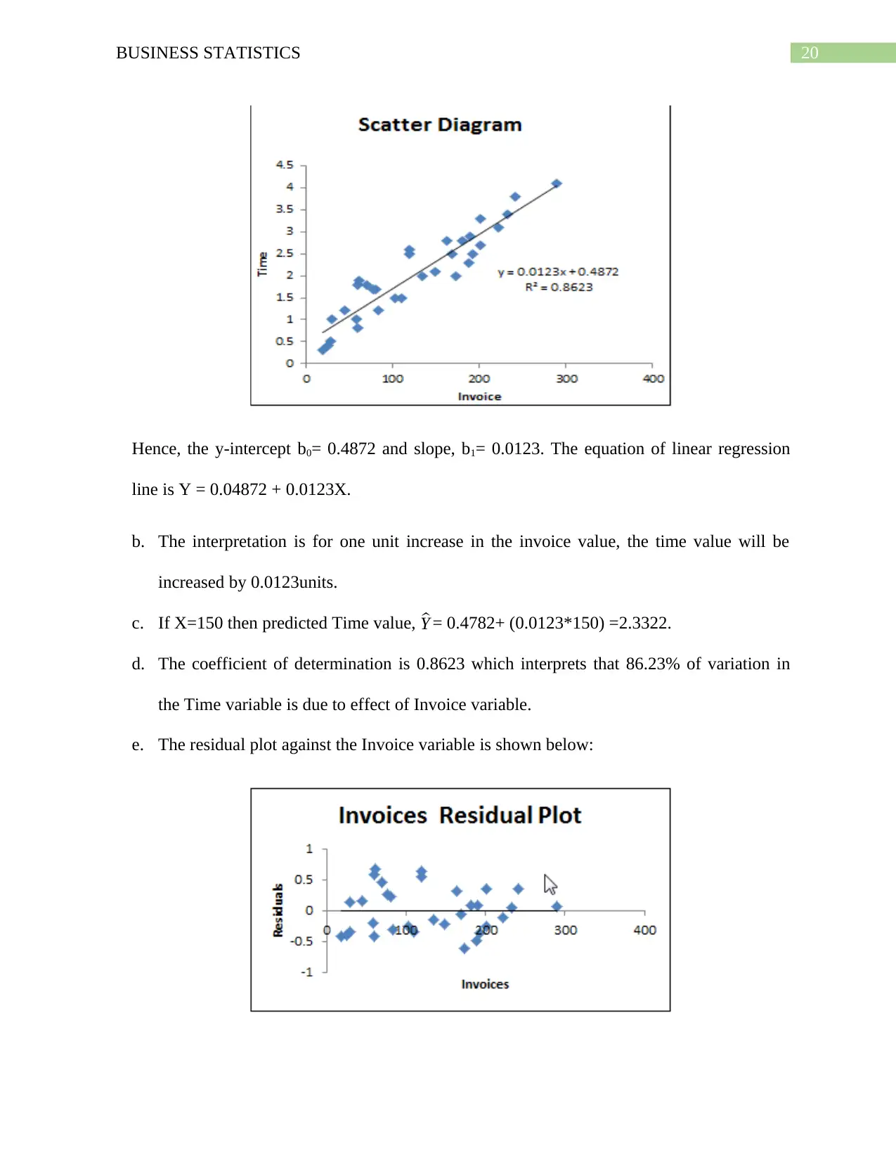
a. The ‘Invoice’ is taken as the independent variable and ‘Time’ as the dependent variable.
To calculate the regression coefficients b0 and b1, the Data Analysis Tool Pak of the MS-
Excel can be used and the scatter diagram is plotted.
20BUSINESS STATISTICS
Hence, the y-intercept b0= 0.4872 and slope, b1= 0.0123. The equation of linear regression
line is Y = 0.04872 + 0.0123X.
b. The interpretation is for one unit increase in the invoice value, the time value will be
increased by 0.0123units.
c. If X=150 then predicted Time value, ^Y = 0.4782+ (0.0123*150) =2.3322.
d. The coefficient of determination is 0.8623 which interprets that 86.23% of variation in
the Time variable is due to effect of Invoice variable.
e. The residual plot against the Invoice variable is shown below:
21BUSINESS STATISTICS
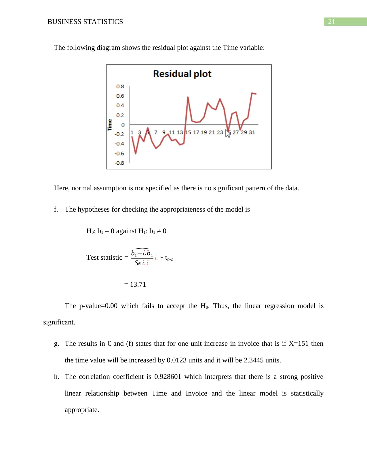
The following diagram shows the residual plot against the Time variable:
Here, normal assumption is not specified as there is no significant pattern of the data.
f. The hypotheses for checking the appropriateness of the model is
H0: b1 = 0 against H1: b1 ≠ 0
Test statistic = ^b1−¿ b1
Se ¿ ¿ ¿ ~ tn-2
= 13.71
The p-value=0.00 which fails to accept the H0. Thus, the linear regression model is
significant.
g. The results in € and (f) states that for one unit increase in invoice that is if X=151 then
the time value will be increased by 0.0123 units and it will be 2.3445 units.
h. The correlation coefficient is 0.928601 which interprets that there is a strong positive
linear relationship between Time and Invoice and the linear model is statistically
appropriate.
Secure Best Marks with AI Grader
Need help grading? Try our AI Grader for instant feedback on your assignments.
22BUSINESS STATISTICS
Response to Question 12.81.
The number of wins is the dependent variable and the independent variable is ERA.
a. The regression equation is obtained in MS Excel.
Coefficien
ts
Standar
d Error t Stat P-value
Lower
95%
Upper
95%
Lower
95.0%
Upper
95.0%
Interce
pt 168.7804
14.8138
6
11.3934
1
5.01E-
12
138.435
5
199.125
2
138.435
5
199.125
2
E.R.A.
(X) -22.7194
3.81421
4
-
5.95652
2.06E-
06
-
30.5325
-
14.9064
-
30.5325
-
14.9064
The intercept b0= 168.7804, slope b1= -22.7194. The regression equation is
Wins = 168.7804 – 22.7194 ERA.
b. The intercept value 168.7804 is a constant value which is not altered due to the positive
or negative change in ERA. The one unit increase in ERA implies 22.7194 unit decrease
in Wins value.
c. For X = 4.50, the predicted value of Wins, ^Y = 168.7804 – (22.7194 *4.50) = 66.5431≈
67.
d. The coefficient of determination 0.5589 which states that 56% variability of wins is
explained by the ERA.
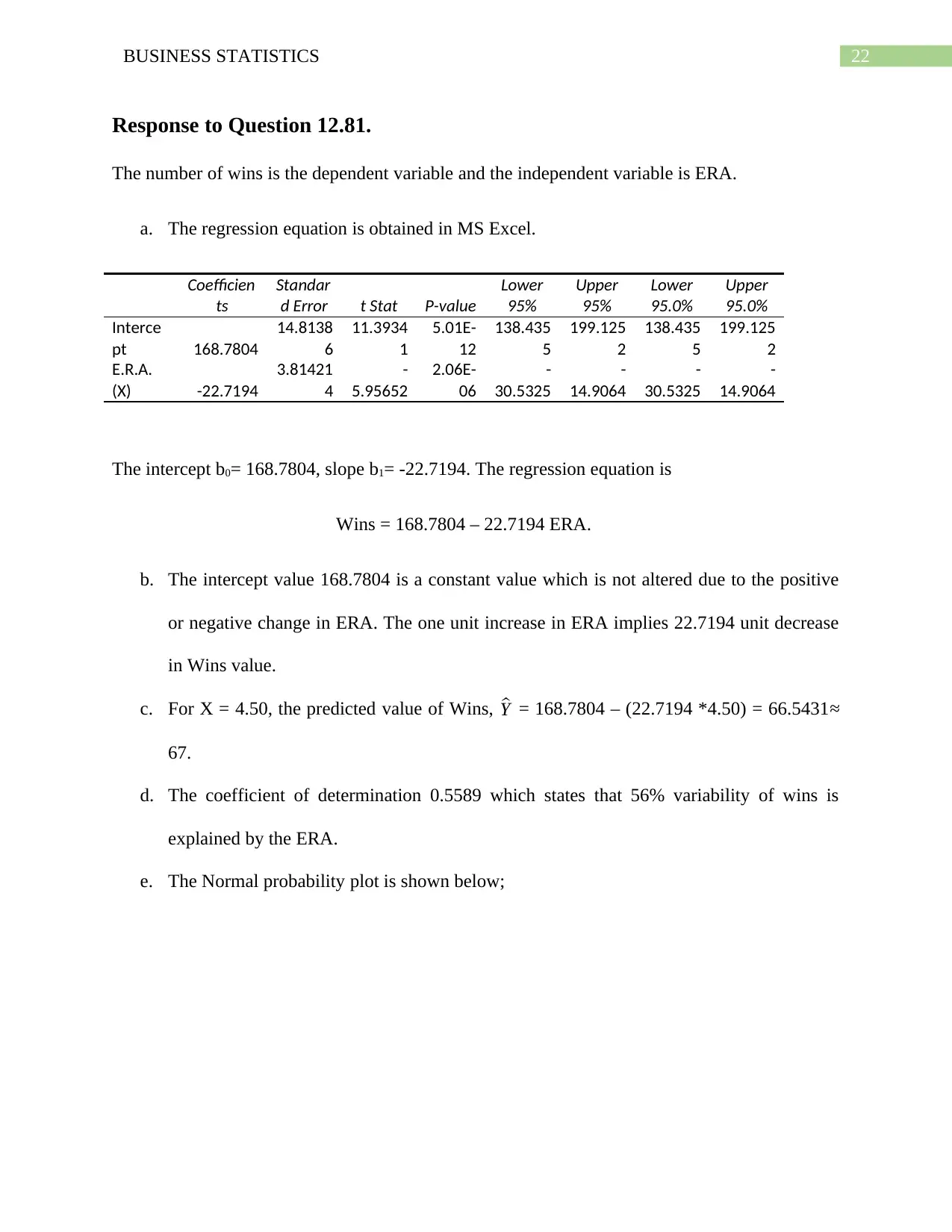
e. The Normal probability plot is shown below;
23BUSINESS STATISTICS
0 20 40 60 80 100 120
0
50
100
150
Normal Probability Plot
Sample Percentile
Wins(Y)
The scattered points have less variability around the least square line and there is no outlier.
Moreover, the trendline is linear.
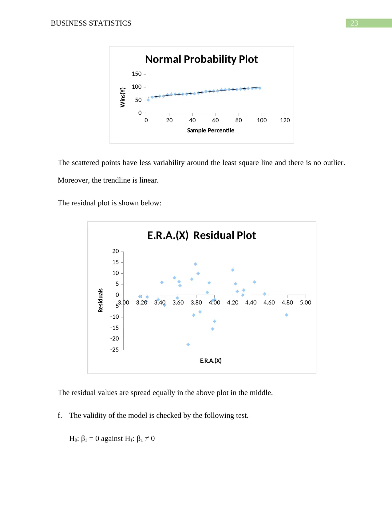
The residual plot is shown below:
3.00 3.20 3.40 3.60 3.80 4.00 4.20 4.40 4.60 4.80 5.00
-25
-20
-15
-10
-5
0
5
10
15
20
E.R.A.(X) Residual Plot
E.R.A.(X)
Residuals
The residual values are spread equally in the above plot in the middle.
f. The validity of the model is checked by the following test.
H0: β1 = 0 against H1: β1 ≠ 0
24BUSINESS STATISTICS
The p-value is 0.00 at 5% level of significance which shows that the null hypothesis is
rejected and there is linear relationship between the Wins and ERA.
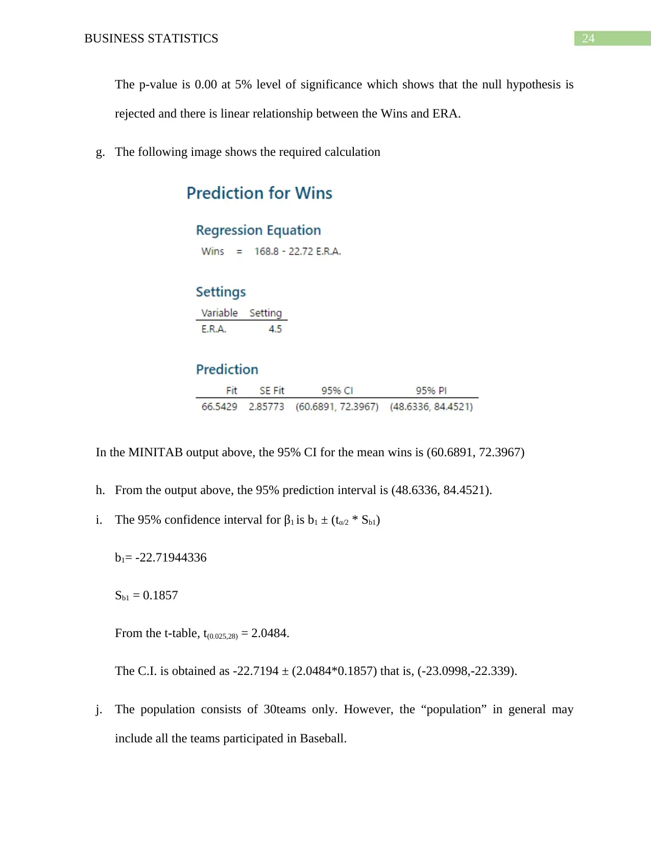
g. The following image shows the required calculation
In the MINITAB output above, the 95% CI for the mean wins is (60.6891, 72.3967)
h. From the output above, the 95% prediction interval is (48.6336, 84.4521).
i. The 95% confidence interval for β1 is b1 ± (tα/2 * Sb1)
b1= -22.71944336
Sb1 = 0.1857
From the t-table, t(0.025,28) = 2.0484.
The C.I. is obtained as -22.7194 ± (2.0484*0.1857) that is, (-23.0998,-22.339).
j. The population consists of 30teams only. However, the “population” in general may
include all the teams participated in Baseball.
Paraphrase This Document
Need a fresh take? Get an instant paraphrase of this document with our AI Paraphraser
25BUSINESS STATISTICS
k. The other independent variables considered in the model are League and Runs Scored per
Game.
l. The results from (a) to (k) shows that the ERA is a useful predictor on the number of
wins. The linear relationship is negative and the regression line is a good fit.
Response to Question 13.49.
a. The given regression equation gives the predicted purchase behavior value for X1 = X2 =
2 as ^Y i = -3.888 + (1.449 ×2) + (1.462×2) – (0.19×2×2) = 1.174.
b. If X1 = 2 and X2 = 7 then the predicted equation is ^Y i = -3.888 + (1.449×2) + (1.462×7) –
(0.19×2×7) = 6.584.
c. The predicted Y value for X1 = 7 and X2 = 2 is ^Y i = -3.888 + (1.449 ×7) + (1.462 ×2) –
(0.19×7×2) = 6.519.
d. The predicted purchase behavior when X1 = 7 and X2 = 7, is ^Y i = -3.888 + (1.449×7) +
(1.462×7) – (0.19×7×7) = 7.179.
e. The slope of X1 when X2 = 2 is calculated as, ^Y i = -3.888 + (1.449× X1i) + (1.462 ×2) –
(0.19×2 × X1i) = -0.964 + 1.069 X1i.
Thus, the slope of X1 is 1.069 when X2 is 2.
f. The regression equation for X2 = 7 is ^Y i = -3.888 + (1.449× X1i) + (1.462×7) – (0.19×7 ×
X1i) = 6.346 + 0.119 X1i.
The slope of X1 is 0.119.
g. The regression equation for X1 =2 is ^Y i = -3.888 + (1.449 ×2) + (1.462 × X2i) – (0.19 ×2 ×
X2i) = -0.99 + 1.082 X2i.
26BUSINESS STATISTICS
The slope of X2 is 1.082.
h. The regression equation for X1 = 7 is
^Y i = -3.888 + (1.449 ×7) + (1.462 × X2i) – (0.19×7 × X2i) = 6.255+0.132 X2i and the slope of
X2 is 0.132.
i. From parts (e) to (f), it can be observed that with the increase of X2 variable from 2 to 7,
the value of X1 variable decreases from 1.069 to 0.119. Thus, the effect of one
independent variable X1 on the dependent variable decreases as the value of the other
variable X2 increases.
From part (g) to (h), the slope of the X2 variable reduces from 1.082 to 0.132 as X1
increases from 2 to 7. Hence, , the effect of one independent variable X2 on the dependent
variable decreases as the value of the other variable X1 increases.
The predicted purchase behavior increases from 1.174 to 6.584 as X2 increases from 2 to
7, remaining the value of X1 at 2 for parts (a) and (b). From (a) and (c), the ^Y i increase
from 1.174 to 6.519. However, in parts (b) and (d), ^Y i increases to a very small extent.
This happens due to negative effect.
Response to Question 13.51.
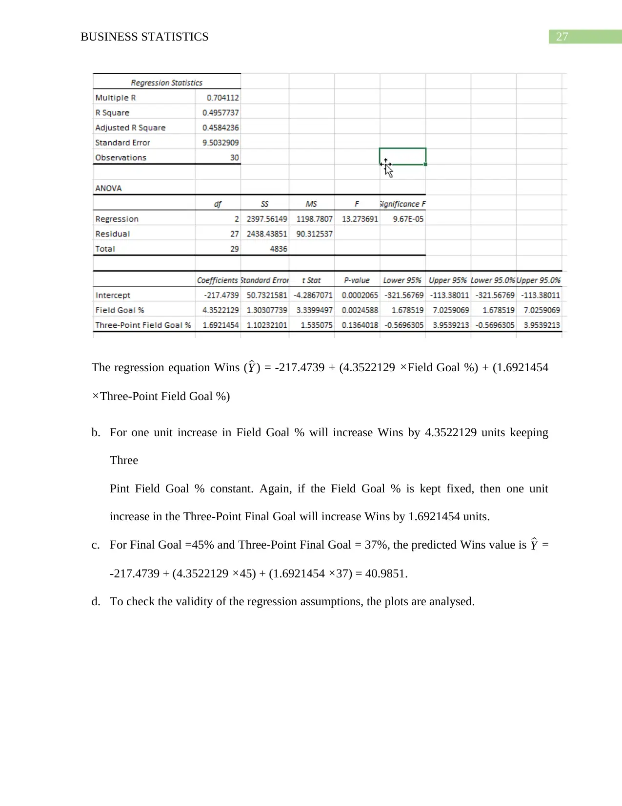
a. The multiple regression line can be calculated in MS Excel using the steps Data Data
Analysis Regression.
27BUSINESS STATISTICS
The regression equation Wins ( ^Y ) = -217.4739 + (4.3522129 ×Field Goal %) + (1.6921454
×Three-Point Field Goal %)
b. For one unit increase in Field Goal % will increase Wins by 4.3522129 units keeping
Three
Pint Field Goal % constant. Again, if the Field Goal % is kept fixed, then one unit
increase in the Three-Point Final Goal will increase Wins by 1.6921454 units.
c. For Final Goal =45% and Three-Point Final Goal = 37%, the predicted Wins value is ^Y =
-217.4739 + (4.3522129 ×45) + (1.6921454 ×37) = 40.9851.
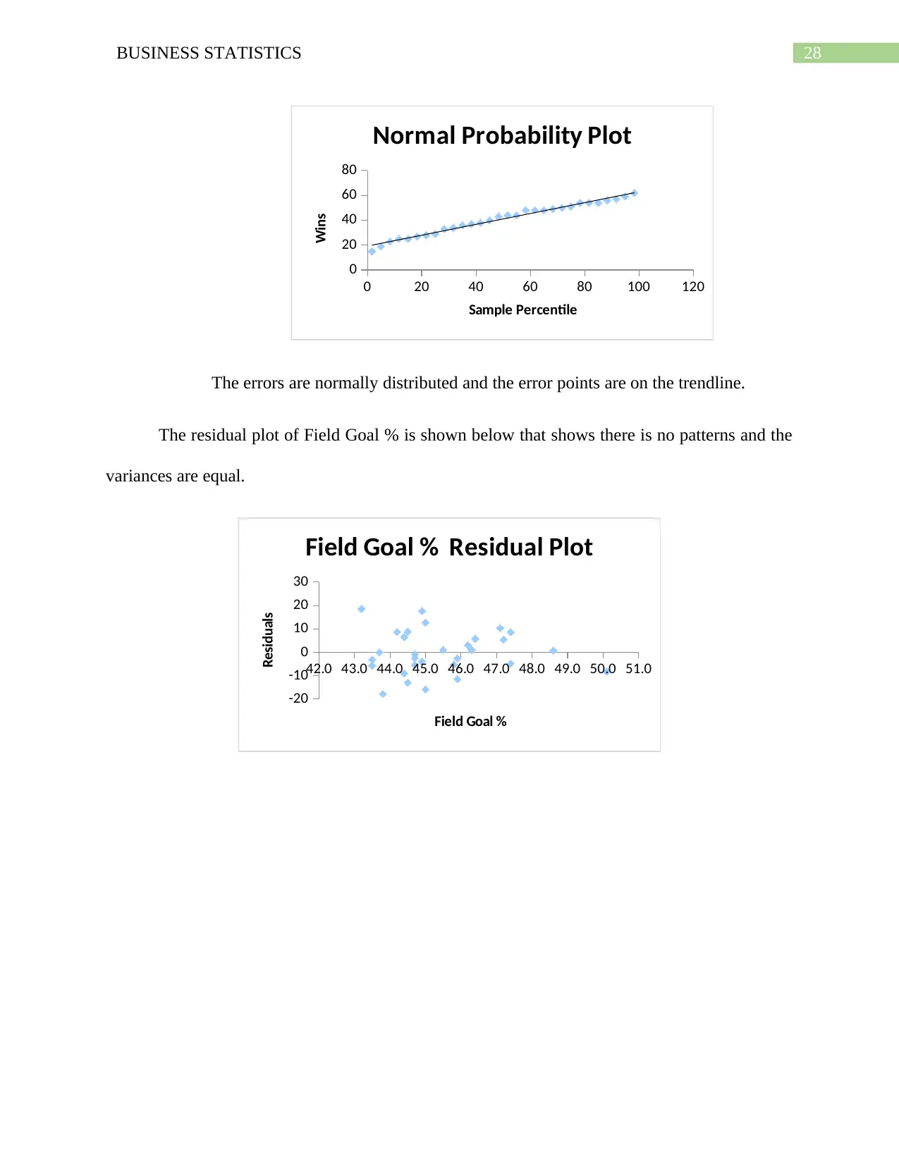
d. To check the validity of the regression assumptions, the plots are analysed.
Secure Best Marks with AI Grader
Need help grading? Try our AI Grader for instant feedback on your assignments.
28BUSINESS STATISTICS
0 20 40 60 80 100 120
0
20
40
60
80
Normal Probability Plot
Sample Percentile
Wins
The errors are normally distributed and the error points are on the trendline.
The residual plot of Field Goal % is shown below that shows there is no patterns and the
variances are equal.
42.0 43.0 44.0 45.0 46.0 47.0 48.0 49.0 50.0 51.0
-20
-10
0
10
20
30
Field Goal % Residual Plot
Field Goal %
Residuals
29BUSINESS STATISTICS
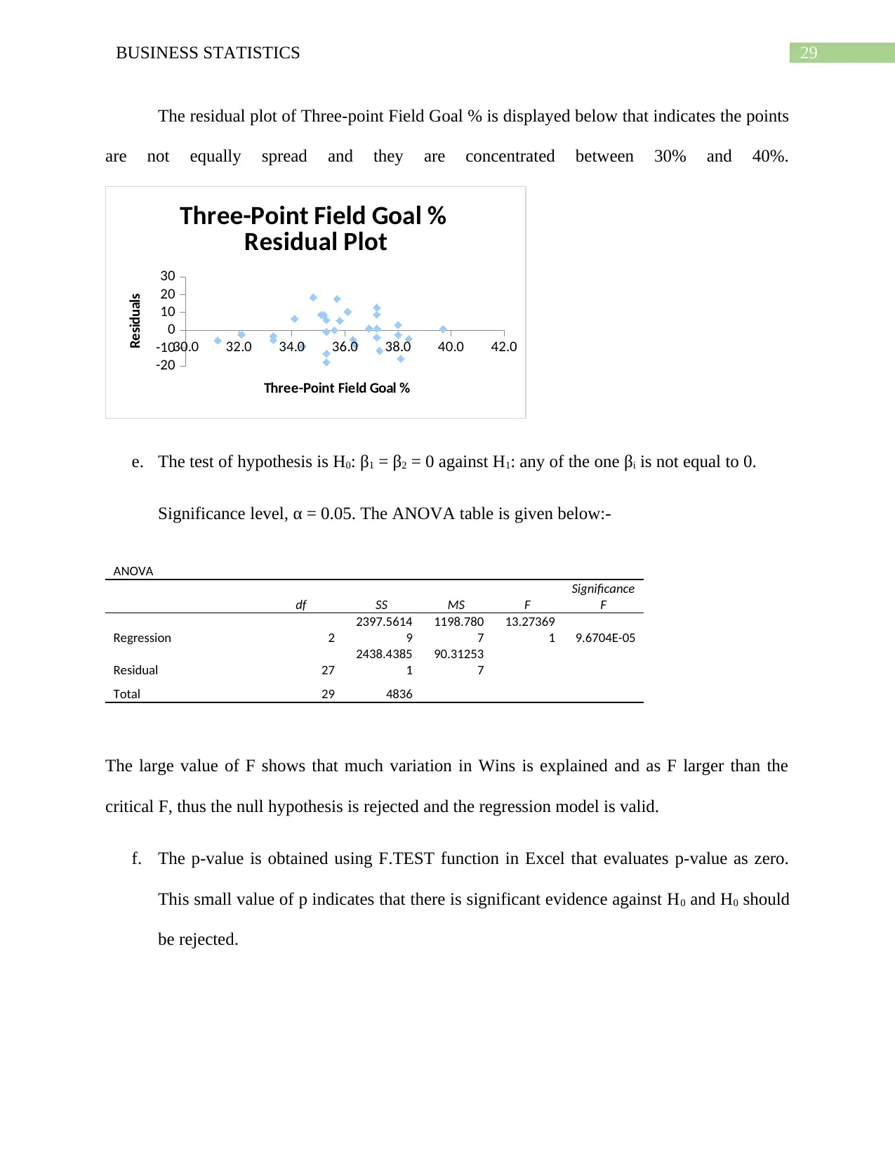
The residual plot of Three-point Field Goal % is displayed below that indicates the points
are not equally spread and they are concentrated between 30% and 40%.
30.0 32.0 34.0 36.0 38.0 40.0 42.0
-20
-10
0
10
20
30
Three-Point Field Goal %
Residual Plot
Three-Point Field Goal %
Residuals
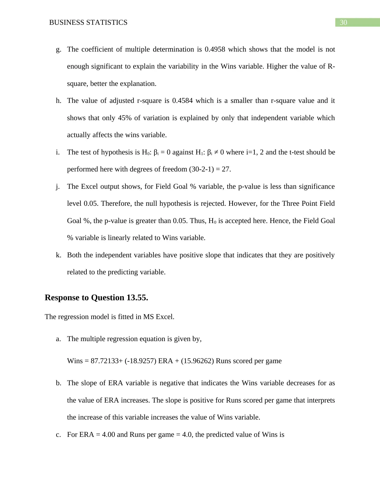
e. The test of hypothesis is H0: β1 = β2 = 0 against H1: any of the one βi is not equal to 0.
Significance level, α = 0.05. The ANOVA table is given below:-
ANOVA
df SS MS F
Significance
F
Regression 2
2397.5614
9
1198.780
7
13.27369
1 9.6704E-05
Residual 27
2438.4385
1
90.31253
7
Total 29 4836
The large value of F shows that much variation in Wins is explained and as F larger than the
critical F, thus the null hypothesis is rejected and the regression model is valid.
f. The p-value is obtained using F.TEST function in Excel that evaluates p-value as zero.
This small value of p indicates that there is significant evidence against H0 and H0 should
be rejected.
30BUSINESS STATISTICS
g. The coefficient of multiple determination is 0.4958 which shows that the model is not
enough significant to explain the variability in the Wins variable. Higher the value of R-
square, better the explanation.
h. The value of adjusted r-square is 0.4584 which is a smaller than r-square value and it
shows that only 45% of variation is explained by only that independent variable which
actually affects the wins variable.
i. The test of hypothesis is H0: βi = 0 against H1: βi ≠ 0 where i=1, 2 and the t-test should be
performed here with degrees of freedom (30-2-1) = 27.
j. The Excel output shows, for Field Goal % variable, the p-value is less than significance
level 0.05. Therefore, the null hypothesis is rejected. However, for the Three Point Field
Goal %, the p-value is greater than 0.05. Thus, H0 is accepted here. Hence, the Field Goal
% variable is linearly related to Wins variable.
k. Both the independent variables have positive slope that indicates that they are positively
related to the predicting variable.
Response to Question 13.55.
The regression model is fitted in MS Excel.
a. The multiple regression equation is given by,
Wins = 87.72133+ (-18.9257) ERA + (15.96262) Runs scored per game
b. The slope of ERA variable is negative that indicates the Wins variable decreases for as
the value of ERA increases. The slope is positive for Runs scored per game that interprets
the increase of this variable increases the value of Wins variable.
c. For ERA = 4.00 and Runs per game = 4.0, the predicted value of Wins is
Paraphrase This Document
Need a fresh take? Get an instant paraphrase of this document with our AI Paraphraser
31BUSINESS STATISTICS
^Wins = 87.72133- (18.9257 ×4) + (15.96262 ×4) = 63.85048 – 75.7028 + 87.72133 =
75.86901 ≈ 76.
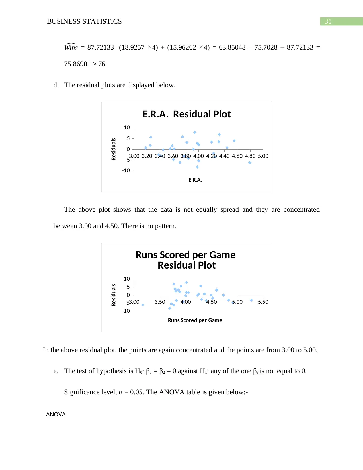
d. The residual plots are displayed below.
3.00 3.20 3.40 3.60 3.80 4.00 4.20 4.40 4.60 4.80 5.00
-10
-5
0
5
10
E.R.A. Residual Plot
E.R.A.
Residuals
The above plot shows that the data is not equally spread and they are concentrated
between 3.00 and 4.50. There is no pattern.
3.00 3.50 4.00 4.50 5.00 5.50
-10
-5
0
5
10
Runs Scored per Game
Residual Plot
Runs Scored per Game
Residuals
In the above residual plot, the points are again concentrated and the points are from 3.00 to 5.00.
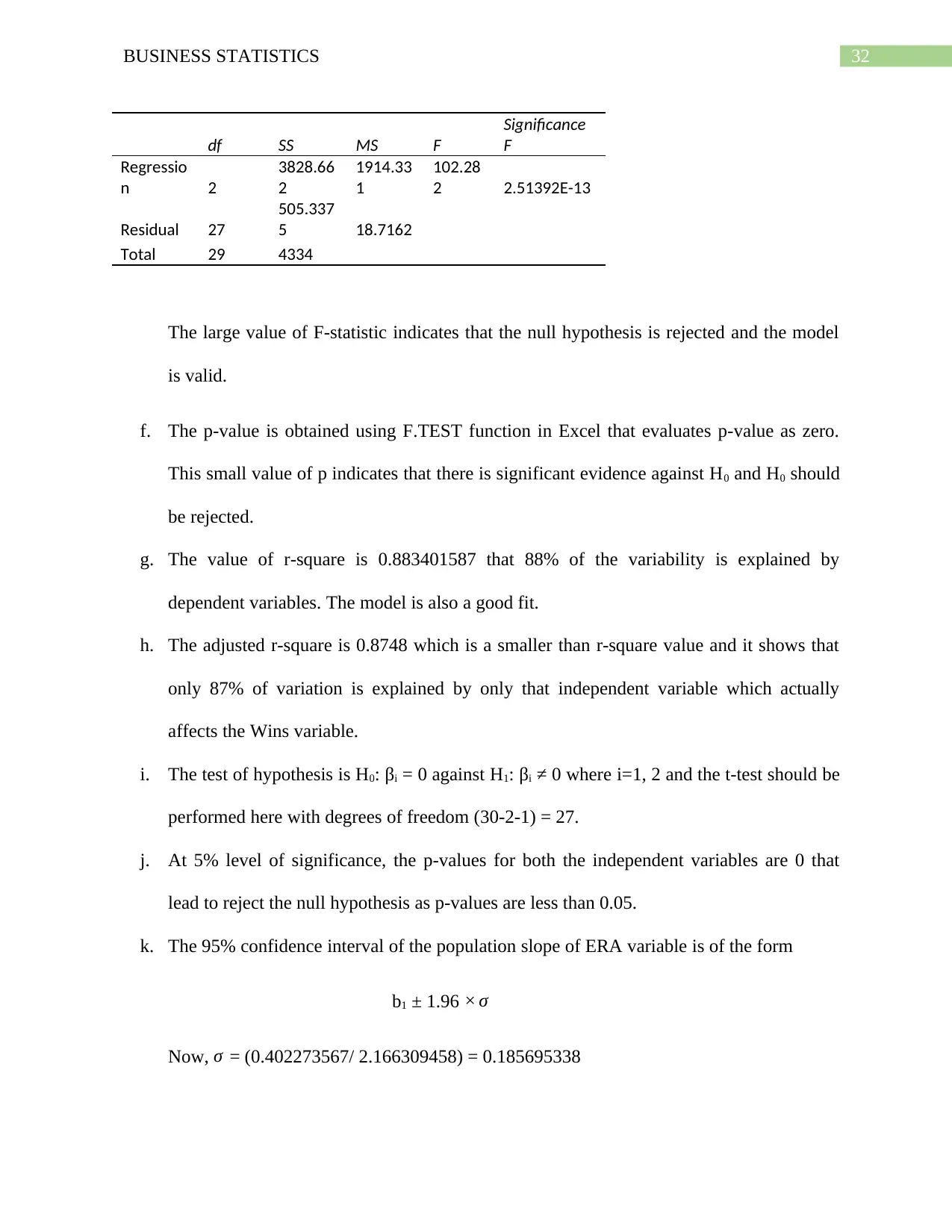
e. The test of hypothesis is H0: β1 = β2 = 0 against H1: any of the one βi is not equal to 0.
Significance level, α = 0.05. The ANOVA table is given below:-
ANOVA
32BUSINESS STATISTICS
df SS MS F
Significance
F
Regressio
n 2
3828.66
2
1914.33
1
102.28
2 2.51392E-13
Residual 27
505.337
5 18.7162
Total 29 4334
The large value of F-statistic indicates that the null hypothesis is rejected and the model
is valid.
f. The p-value is obtained using F.TEST function in Excel that evaluates p-value as zero.
This small value of p indicates that there is significant evidence against H0 and H0 should
be rejected.
g. The value of r-square is 0.883401587 that 88% of the variability is explained by
dependent variables. The model is also a good fit.
h. The adjusted r-square is 0.8748 which is a smaller than r-square value and it shows that
only 87% of variation is explained by only that independent variable which actually
affects the Wins variable.
i. The test of hypothesis is H0: βi = 0 against H1: βi ≠ 0 where i=1, 2 and the t-test should be
performed here with degrees of freedom (30-2-1) = 27.
j. At 5% level of significance, the p-values for both the independent variables are 0 that
lead to reject the null hypothesis as p-values are less than 0.05.
k. The 95% confidence interval of the population slope of ERA variable is of the form
b1 ± 1.96 × σ
Now, σ = (0.402273567/ 2.166309458) = 0.185695338
33BUSINESS STATISTICS
The 95% C.I. is ((-18.9257) ± 1.96 × 0.185695) that is, (-19.28966, -18.56174).
l. The absolute value of the coefficient actually determines the importance of the predictor
in the regression model. IN this problem, the mod value of the coefficient of ERA is
larger than that of Runs scored per game. Thus, the pitching, as measured by ERA is
more important in predicting wins.s
1 out of 34
Related Documents
Your All-in-One AI-Powered Toolkit for Academic Success.
+13062052269
info@desklib.com
Available 24*7 on WhatsApp / Email
![[object Object]](/_next/static/media/star-bottom.7253800d.svg)
Unlock your academic potential
© 2024 | Zucol Services PVT LTD | All rights reserved.


