BUSINESS STATISTICS.

BUSINESS STATISTICS
STUDENT ID:
[Pick the date]
[Type the abstract of the document here. The abstract is typically a short summary of the contents
of the document. Type the abstract of the document here. The abstract is typically a short
summary of the contents of the document.]

Assignment Part I
Task 1
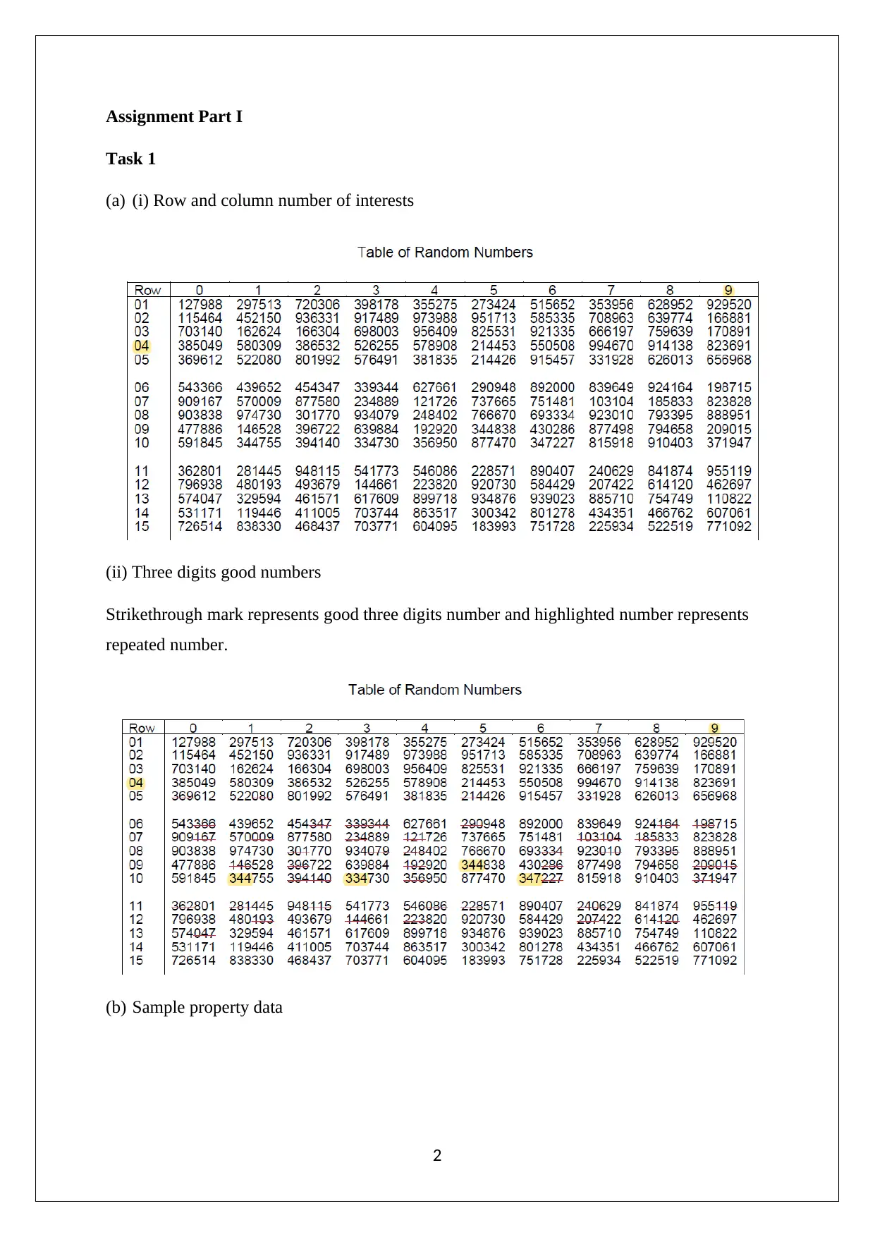
(a) (i) Row and column number of interests
(ii) Three digits good numbers
Strikethrough mark represents good three digits number and highlighted number represents
repeated number.
(b) Sample property data
2

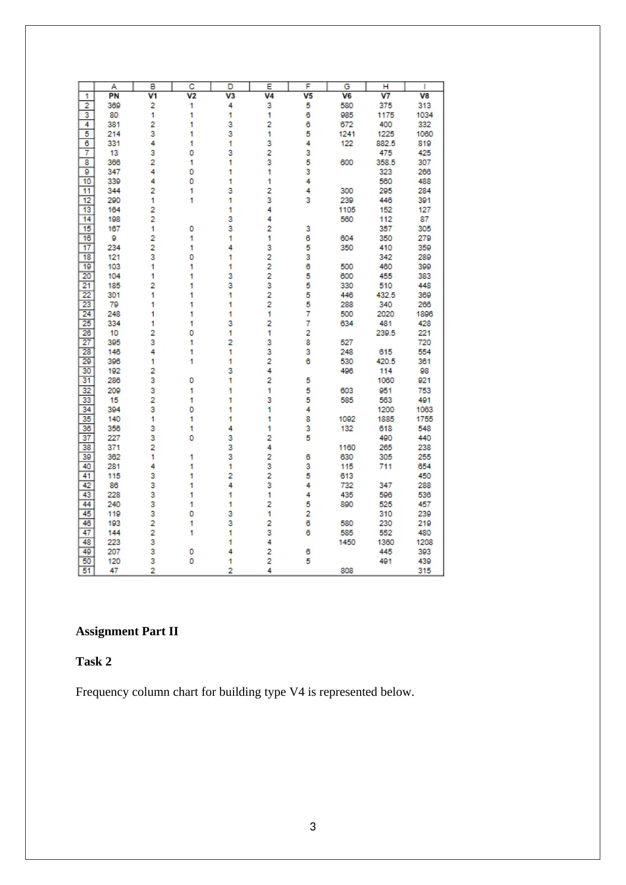
Assignment Part II
Task 2
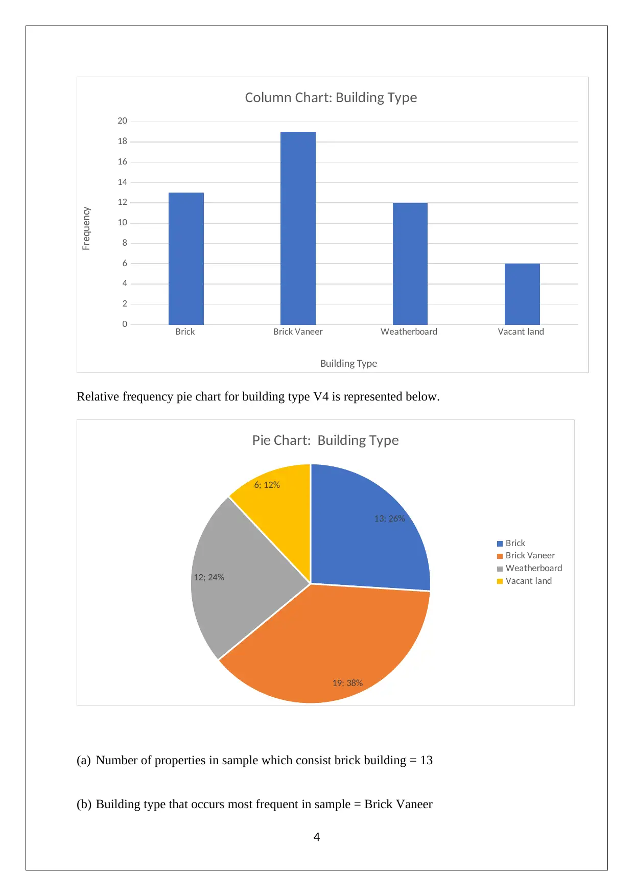
Frequency column chart for building type V4 is represented below.
3

Brick Brick Vaneer Weatherboard Vacant land
0
2
4
6
8
10
12
14
16
18
20
Column Chart: Building Type
Building Type
Frequency
Relative frequency pie chart for building type V4 is represented below.
13; 26%
19; 38%
12; 24%
6; 12%
Pie Chart: Building Type
Brick
Brick Vaneer
Weatherboard
Vacant land
(a) Number of properties in sample which consist brick building = 13
(b) Building type that occurs most frequent in sample = Brick Vaneer
4

(c) Proportion of properties in sample which consist weatherboard building = 0.24
Task 3
Sorted ‘Sold Price’ (V7) data in ascending order is highlighted below.
5

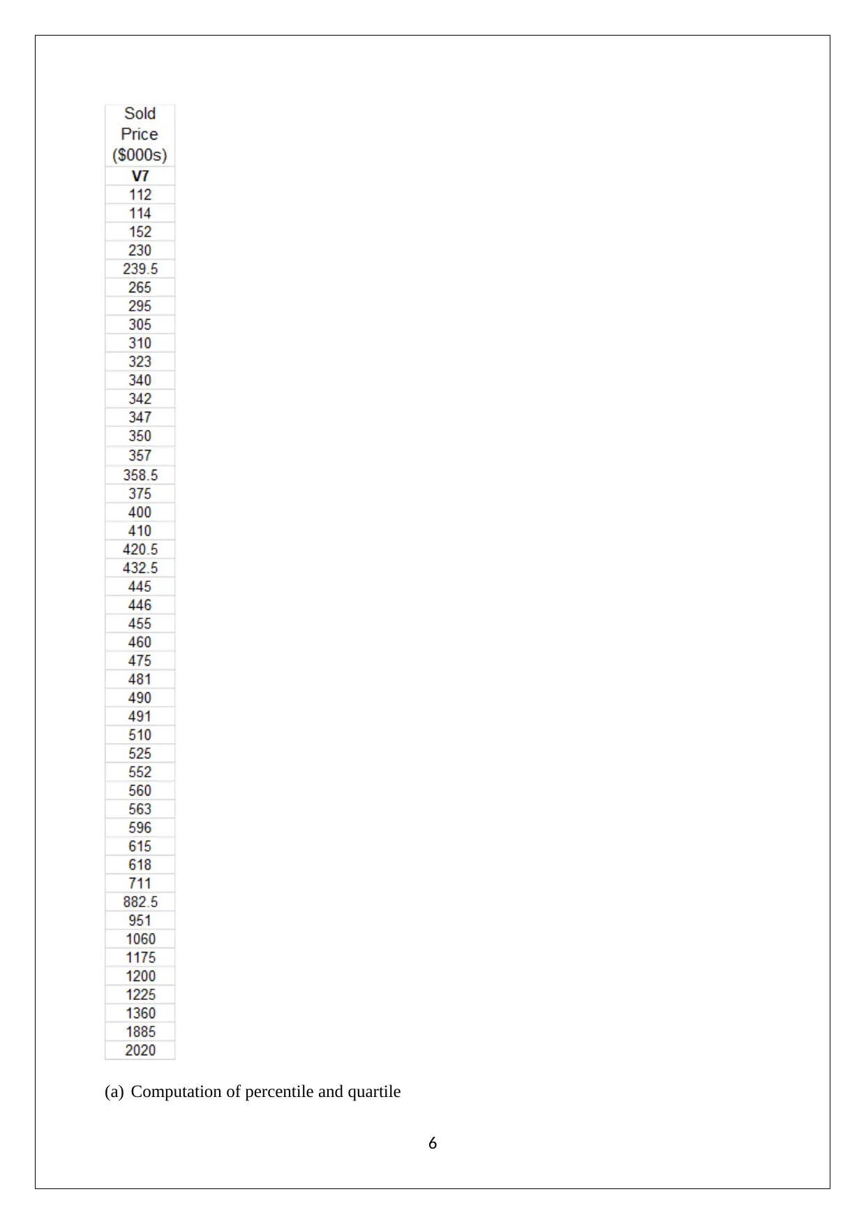
(a) Computation of percentile and quartile
6

(i) Percentile location formula
Lp=P ( n+1 )
100
Where, P = Required percentile value
n= number of samples
Now,
70th percentile is computed as shown below.
P = 70 and n = 50
L70=70 (50+ 1 )
100
L70=35.7 thterm value
L70=36 thterm value
L70=615
Therefore, the 70th percentile of sold prices comes out to be $615000.
(ii) First and third quartile
Firstquartile (Q1)
The firstquartile is 25ththe percentile.
Percentile location formula
P = 20 and n = 50
Lp=P ( n+1 )
100
Lp=25 ( 50+1 )
100
Lp=12.7 thterm value
Lp=13th term value
L25=347
Hence, first quartile would be $347000.
Third quartile (Q3)
The firstquartile is 75th the percentile.
Percentile location formula
P = 75 and n = 50
Lp=P ( n+1 )
100
Lp=75 ( 50+1 )
100
Lp=38.2th term value
Lp=38th term value
L75=711
Hence, third quartile would be $711000.
(b) The 70th percentile represents that 70% of the sample data values of sold price variable
corresponding to sample properties would have values equal to or lower than $615,000.
7

(c) Inter quartile range of sample sold prices is computed below.
The difference between the third quartile and first quartile is the inter quartile range. Hence,
IQR = Q3-Q1
Here,
Q3 = $711,000
Q1 = $347,000
Hence,
IQR = Q3-Q1
IQR = $711000 - $347000
IQR = $364,000
Therefore, the inter quartile range comes out to be $364,000. The value represents that
middle50% of the sample values of the sale price of properties would fall within the interval
of $364,000
Task 4
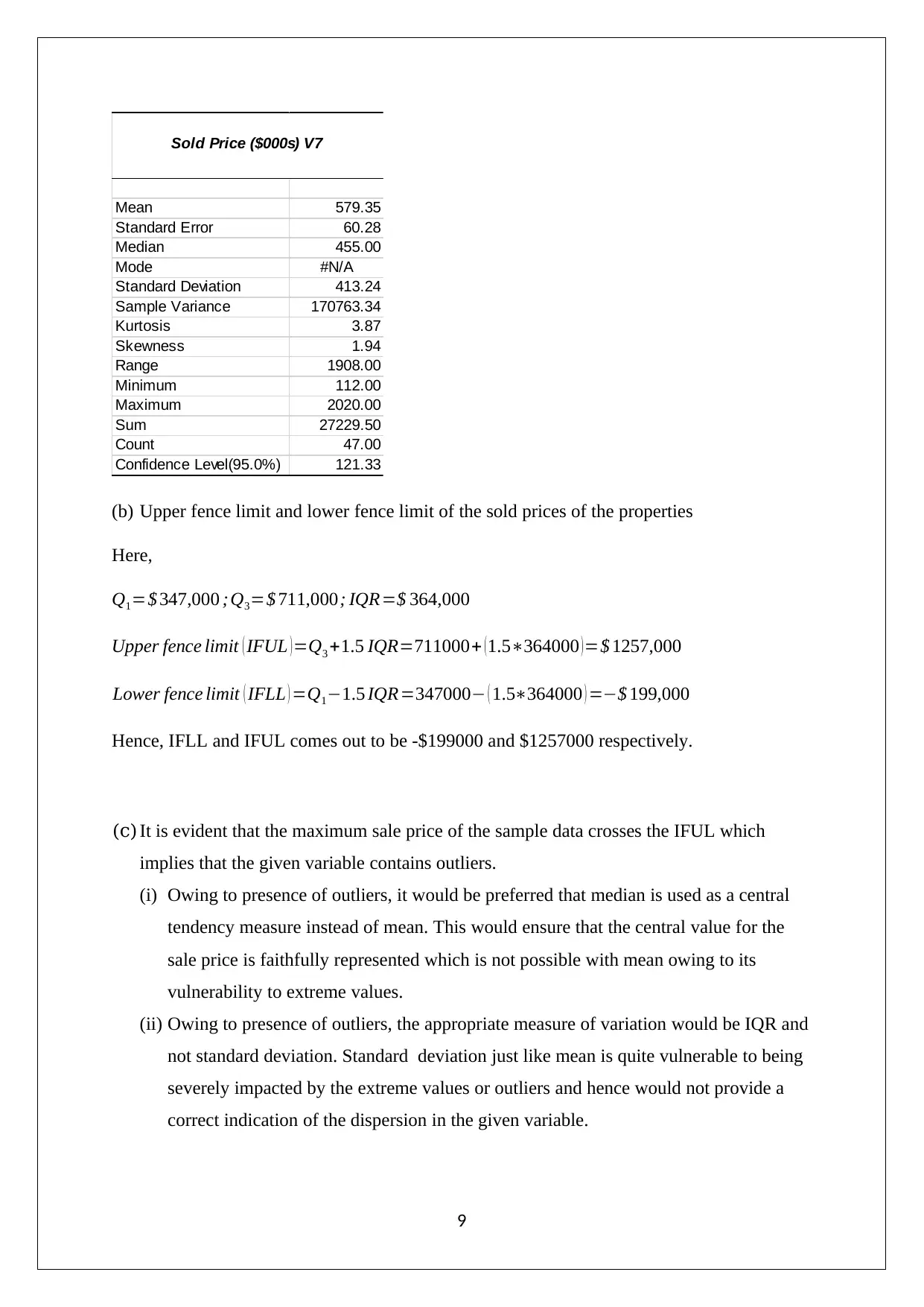
(a) Descriptive statistics of sample sold price of properties has been computed through excel
and the output is shown below.
8

Mean 579.35
Standard Error 60.28
Median 455.00
Mode #N/A
Standard Deviation 413.24
Sample Variance 170763.34
Kurtosis 3.87
Skewness 1.94
Range 1908.00
Minimum 112.00
Maximum 2020.00
Sum 27229.50
Count 47.00
Confidence Level(95.0%) 121.33
Sold Price ($000s) V7
(b) Upper fence limit and lower fence limit of the sold prices of the properties
Here,
Q1=$ 347,000 ;Q3=$ 711,000; IQR=$ 364,000
Upper fence limit ( IFUL ) =Q3 +1.5 IQR=711000+ ( 1.5∗364000 ) =$ 1257,000
Lower fence limit ( IFLL ) =Q1−1.5 IQR=347000− ( 1.5∗364000 ) =−$ 199,000
Hence, IFLL and IFUL comes out to be -$199000 and $1257000 respectively.
(c)It is evident that the maximum sale price of the sample data crosses the IFUL which
implies that the given variable contains outliers.
(i) Owing to presence of outliers, it would be preferred that median is used as a central
tendency measure instead of mean. This would ensure that the central value for the
sale price is faithfully represented which is not possible with mean owing to its
vulnerability to extreme values.
(ii) Owing to presence of outliers, the appropriate measure of variation would be IQR and
not standard deviation. Standard deviation just like mean is quite vulnerable to being
severely impacted by the extreme values or outliers and hence would not provide a
correct indication of the dispersion in the given variable.
9

Task 5
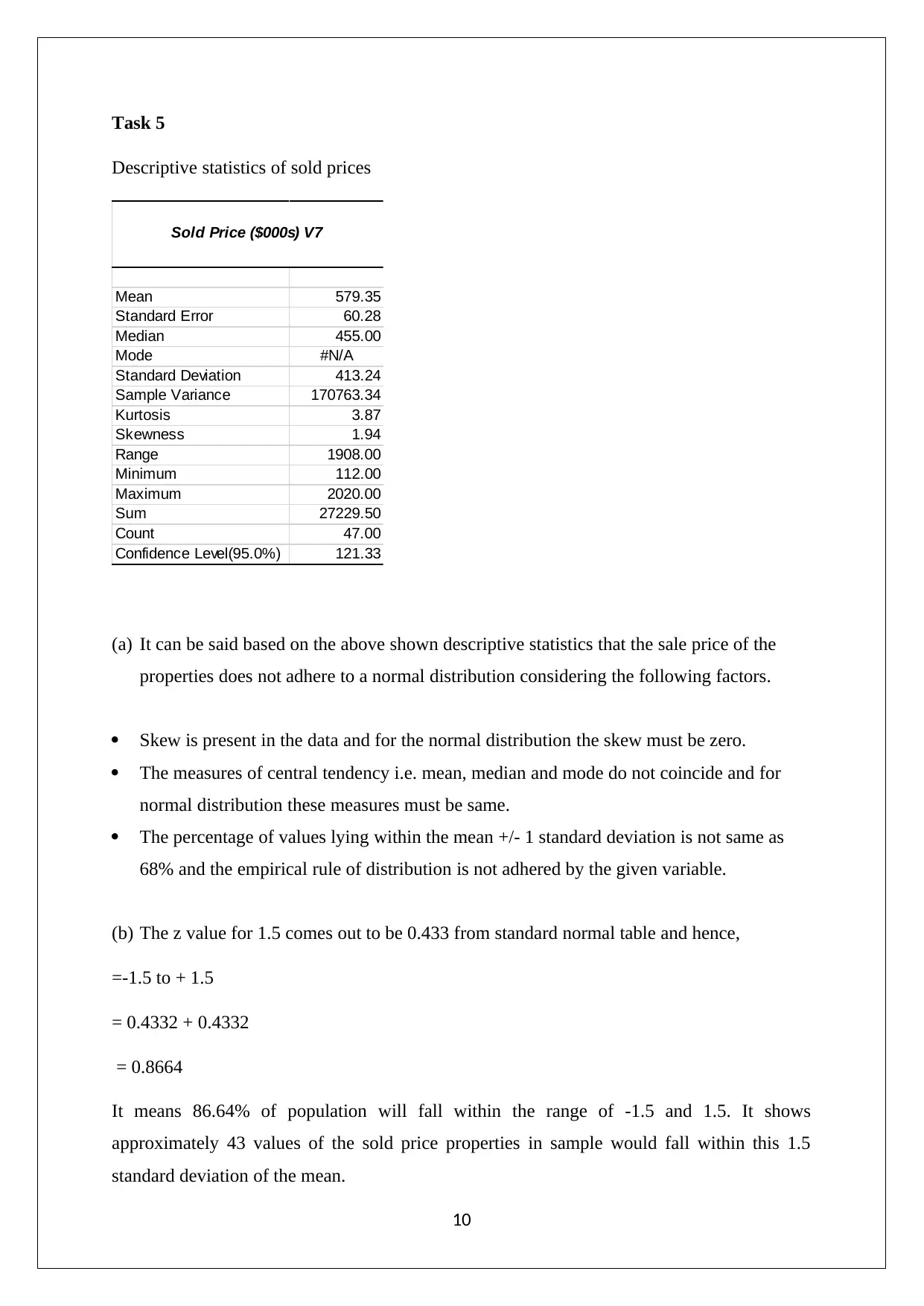
Descriptive statistics of sold prices
Mean 579.35
Standard Error 60.28
Median 455.00
Mode #N/A
Standard Deviation 413.24
Sample Variance 170763.34
Kurtosis 3.87
Skewness 1.94
Range 1908.00
Minimum 112.00
Maximum 2020.00
Sum 27229.50
Count 47.00
Confidence Level(95.0%) 121.33
Sold Price ($000s) V7
(a) It can be said based on the above shown descriptive statistics that the sale price of the
properties does not adhere to a normal distribution considering the following factors.
 Skew is present in the data and for the normal distribution the skew must be zero.
 The measures of central tendency i.e. mean, median and mode do not coincide and for
normal distribution these measures must be same.
 The percentage of values lying within the mean +/- 1 standard deviation is not same as
68% and the empirical rule of distribution is not adhered by the given variable.
(b) The z value for 1.5 comes out to be 0.433 from standard normal table and hence,
=-1.5 to + 1.5
= 0.4332 + 0.4332
= 0.8664
It means 86.64% of population will fall within the range of -1.5 and 1.5. It shows
approximately 43 values of the sold price properties in sample would fall within this 1.5
standard deviation of the mean.
10

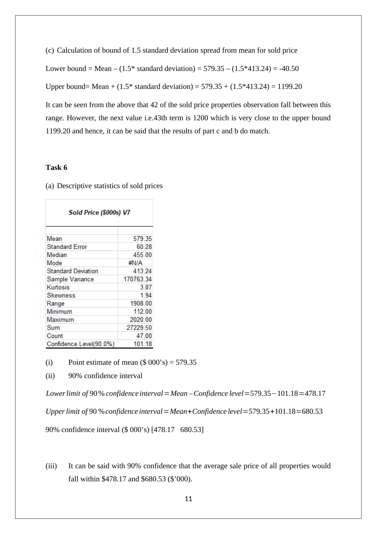
(c) Calculation of bound of 1.5 standard deviation spread from mean for sold price
Lower bound = Mean – (1.5* standard deviation) = 579.35 – (1.5*413.24) = -40.50
Upper bound= Mean + (1.5* standard deviation) = 579.35 + (1.5*413.24) = 1199.20
It can be seen from the above that 42 of the sold price properties observation fall between this
range. However, the next value i.e.43th term is 1200 which is very close to the upper bound
1199.20 and hence, it can be said that the results of part c and b do match.
Task 6
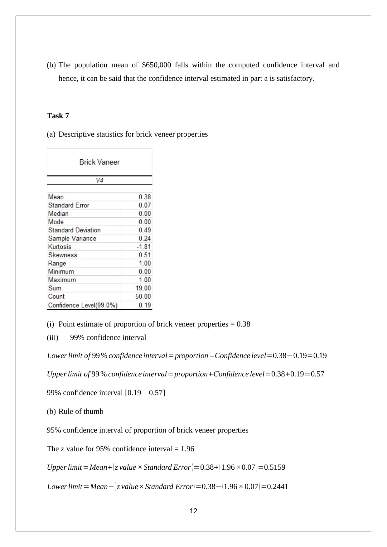
(a) Descriptive statistics of sold prices
(i) Point estimate of mean ($ 000’s) = 579.35
(ii) 90% confidence interval
Lower limit of 90 % confidence interval=Mean – Confidence level=579.35−101.18=478.17
Upper limit of 90 %confidence interval=Mean+Confidence level=579.35+101.18=680.53
90% confidence interval ($ 000’s) [478.17 680.53]
(iii) It can be said with 90% confidence that the average sale price of all properties would
fall within $478.17 and $680.53 ($’000).
11

(b) The population mean of $650,000 falls within the computed confidence interval and
hence, it can be said that the confidence interval estimated in part a is satisfactory.
Task 7
(a) Descriptive statistics for brick veneer properties
(i) Point estimate of proportion of brick veneer properties = 0.38
(iii) 99% confidence interval
Lower limit of 99 % confidence interval=proportion – Confidence level=0.38−0.19=0.19
Upper limit of 99 % confidence interval=proportion+Confidence level=0.38+0.19=0.57
99% confidence interval [0.19 0.57]
(b) Rule of thumb
95% confidence interval of proportion of brick veneer properties
The z value for 95% confidence interval = 1.96
Upper limit =Mean+ ( z value × Standard Error )=0.38+ ( 1.96 ×0.07 )=0.5159
Lower limit =Mean− ( z value× Standard Error ) =0.38− ( 1.96 × 0.07 ) =0.2441
12

By using empirical rule
Upper limit Mean+ ¿
Lower limit =Mean−¿
(c) Based on the above computations, it is apparent that the 99% confidence interval is wider
than the 95% confidence interval. This is on expected lines since the 99% confidence
interval predicts the population mean with higher precision and thereby a wider
confidence interval is desired. The 95% confidence interval estimation does not differ
significantly between the empirical rule and rule of thumb.
13