Business Statistics: Hypothesis Testing

This document provides an overview of hypothesis testing in business statistics. It covers topics such as test statistics, significance level, and interpreting results. The content includes examples and references for further reading.

BUSINESS STATISTICS
ASSIGNMENT 2: HYPOTHESIS TESTING
STUDENT iD:
[Pick the date]

Question 1
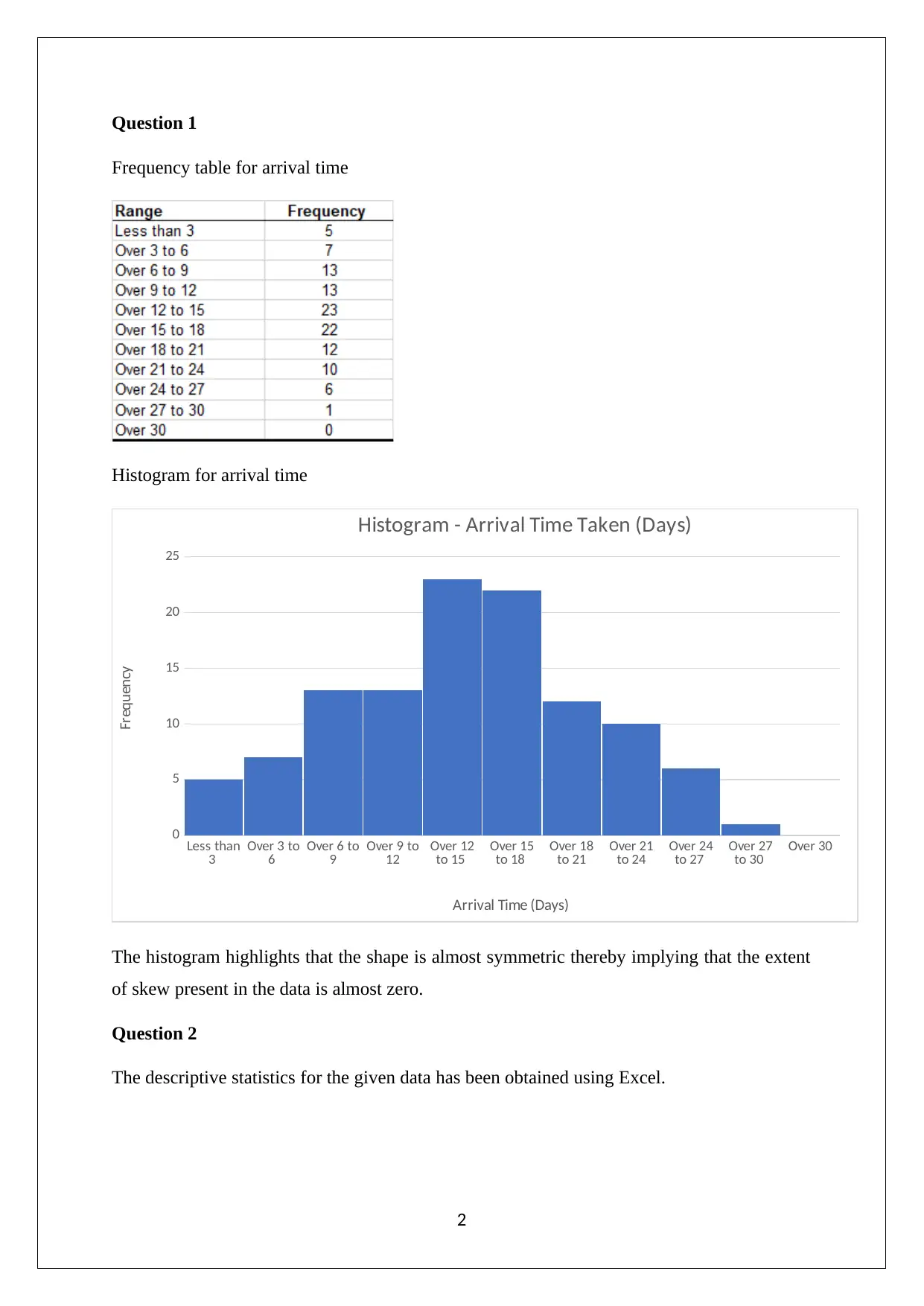
Frequency table for arrival time
Histogram for arrival time
Less than
3 Over 3 to
6 Over 6 to
9 Over 9 to
12 Over 12
to 15 Over 15
to 18 Over 18
to 21 Over 21
to 24 Over 24
to 27 Over 27
to 30 Over 30
0
5
10
15
20
25
Histogram - Arrival Time Taken (Days)
Arrival Time (Days)
Frequency
The histogram highlights that the shape is almost symmetric thereby implying that the extent
of skew present in the data is almost zero.
Question 2
The descriptive statistics for the given data has been obtained using Excel.
2

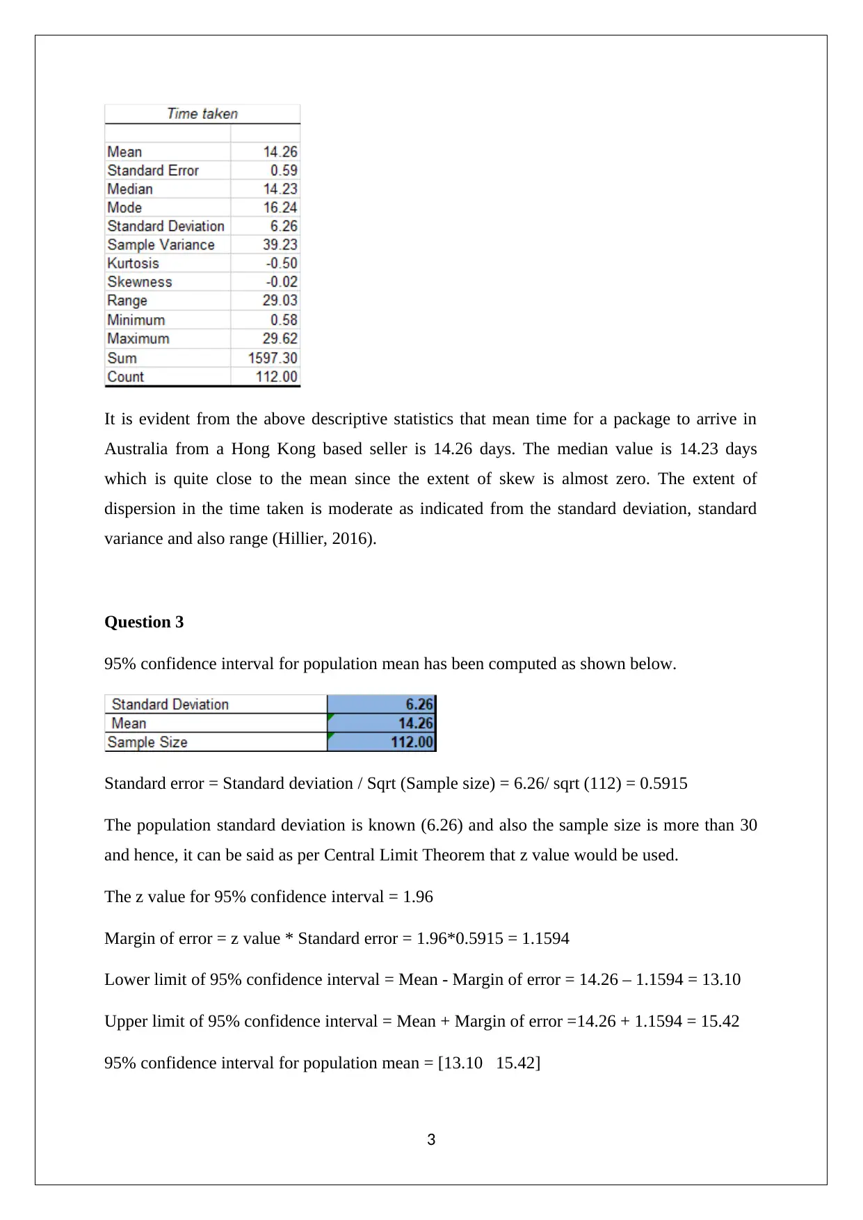
It is evident from the above descriptive statistics that mean time for a package to arrive in
Australia from a Hong Kong based seller is 14.26 days. The median value is 14.23 days
which is quite close to the mean since the extent of skew is almost zero. The extent of
dispersion in the time taken is moderate as indicated from the standard deviation, standard
variance and also range (Hillier, 2016).
Question 3
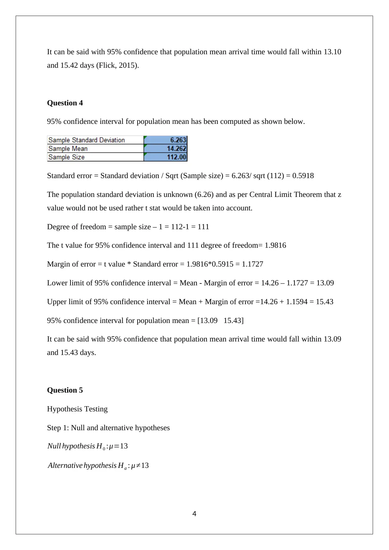
95% confidence interval for population mean has been computed as shown below.
Standard error = Standard deviation / Sqrt (Sample size) = 6.26/ sqrt (112) = 0.5915
The population standard deviation is known (6.26) and also the sample size is more than 30
and hence, it can be said as per Central Limit Theorem that z value would be used.
The z value for 95% confidence interval = 1.96
Margin of error = z value * Standard error = 1.96*0.5915 = 1.1594
Lower limit of 95% confidence interval = Mean - Margin of error = 14.26 – 1.1594 = 13.10
Upper limit of 95% confidence interval = Mean + Margin of error =14.26 + 1.1594 = 15.42
95% confidence interval for population mean = [13.10 15.42]
3

It can be said with 95% confidence that population mean arrival time would fall within 13.10
and 15.42 days (Flick, 2015).
Question 4
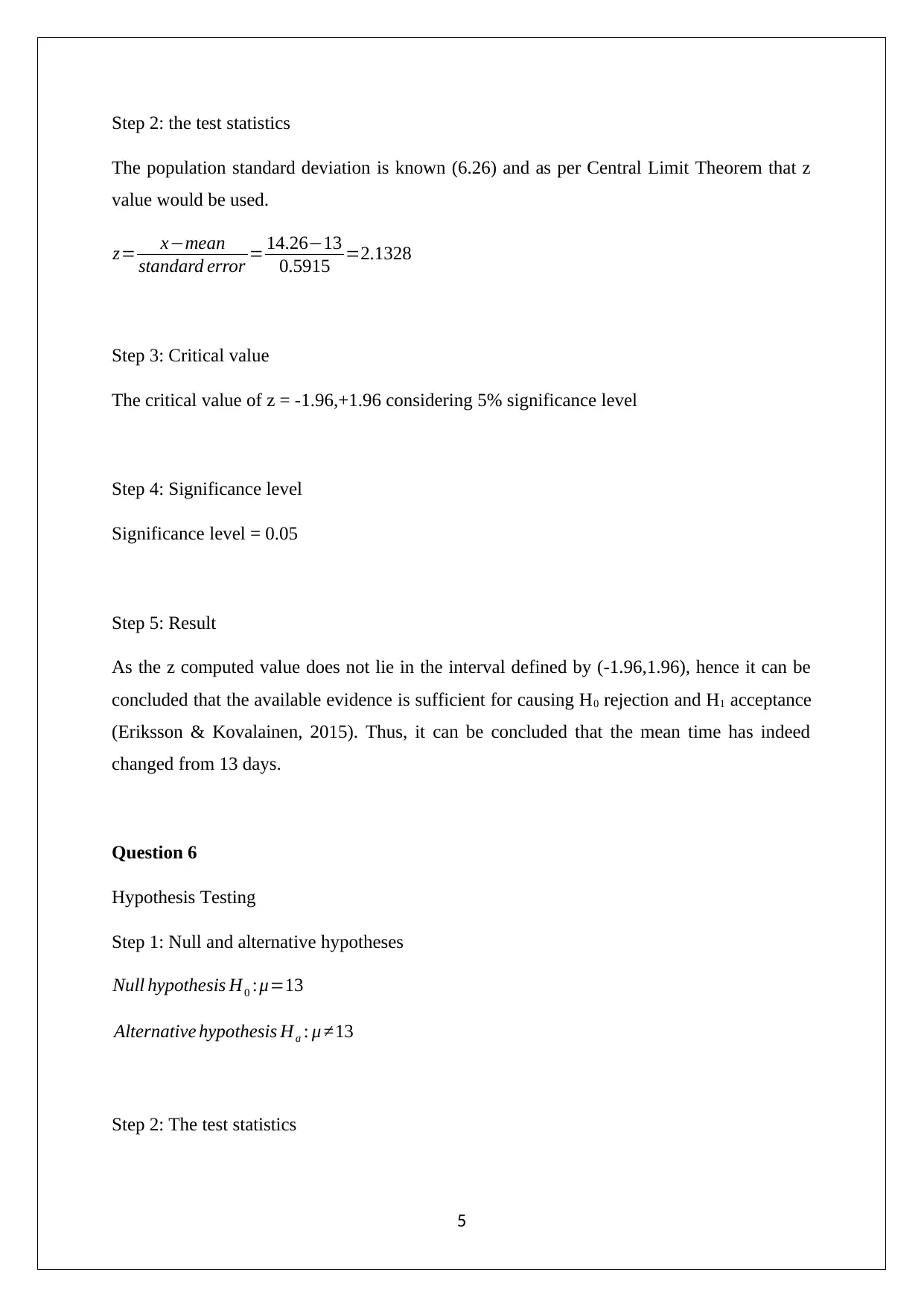
95% confidence interval for population mean has been computed as shown below.
Standard error = Standard deviation / Sqrt (Sample size) = 6.263/ sqrt (112) = 0.5918
The population standard deviation is unknown (6.26) and as per Central Limit Theorem that z
value would not be used rather t stat would be taken into account.
Degree of freedom = sample size – 1 = 112-1 = 111
The t value for 95% confidence interval and 111 degree of freedom= 1.9816
Margin of error = t value * Standard error = 1.9816*0.5915 = 1.1727
Lower limit of 95% confidence interval = Mean - Margin of error = 14.26 – 1.1727 = 13.09
Upper limit of 95% confidence interval = Mean + Margin of error =14.26 + 1.1594 = 15.43
95% confidence interval for population mean = [13.09 15.43]
It can be said with 95% confidence that population mean arrival time would fall within 13.09
and 15.43 days.
Question 5
Hypothesis Testing
Step 1: Null and alternative hypotheses
Null hypothesis H0 :μ=13
Alternative hypothesis Ha : μ ≠13
4

Step 2: the test statistics
The population standard deviation is known (6.26) and as per Central Limit Theorem that z
value would be used.
z= x−mean
standard error = 14.26−13
0.5915 =2.1328
Step 3: Critical value
The critical value of z = -1.96,+1.96 considering 5% significance level
Step 4: Significance level
Significance level = 0.05
Step 5: Result
As the z computed value does not lie in the interval defined by (-1.96,1.96), hence it can be
concluded that the available evidence is sufficient for causing H0 rejection and H1 acceptance
(Eriksson & Kovalainen, 2015). Thus, it can be concluded that the mean time has indeed
changed from 13 days.
Question 6
Hypothesis Testing
Step 1: Null and alternative hypotheses
Null hypothesis H0 :μ=13
Alternative hypothesis Ha : μ ≠13
Step 2: The test statistics
5

The population standard deviation is known (6.26) and as per Central Limit Theorem that z
value would be used.
z= x−mean
standard error = 14.26−13
0.5915 =2.1328
Step 3: The p value
The p value (two tailed)= 0.0352
Step 4: Significance level
Significance level = 0.05
Step 5: Result
It can be said that the p value is lower than the significance (0.0352 <0.05) and hence,
sufficient evidence is sufficient for causing H0 rejection and H1 acceptance (Medhi, 2015).
Thus, it can be concluded that the mean time has indeed changed from 13 days.
Question 7
Hypothesis Testing
Step 1: Null and alternative hypotheses
Null hypothesis H0 :μ ≤ 13
Alternative hypothesis Ha : μ>13
Step 2: The test statistics
The population standard deviation is unknown and hence, t value would be used.
t= x−mean
standard error = 14.26−13
0.5918 =2.1317
6

Step 3: The p value considering df =112-1 = 111
The p value (right tailed) = 0.0176
Step 4: Significance level
Significance level = 0.05
Step 5: Result
It can be said that the p value is lower than the significance (0.0176<0.05) and hence,
sufficient evidence is present to reject the null hypothesis and to accept the alternative
hypothesis. Hence, it can be concluded that population mean value of arrival time is more 13
is correct.
Question 8
The p value indicates the probability of obtaining the underlying results assuming that the
underlying null hypothesis was actually true. If the p value corresponding to the correlation
coefficient is very small, it implies that the underlying result would arrive only when the
correlation coefficient is significant as there is very less probability of the results being
derived owing ti chance (Hastie, Tibshirani & Friedman, 2014).
Question 9
If the p value for one tailed test = 0.03
The p value for two tailed test = 2 * 0.03 = 0.06
Question 10
7

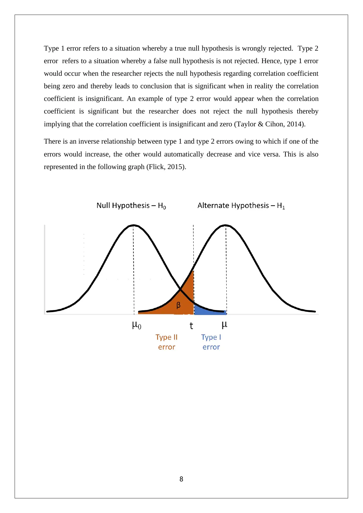
Type 1 error refers to a situation whereby a true null hypothesis is wrongly rejected. Type 2
error refers to a situation whereby a false null hypothesis is not rejected. Hence, type 1 error
would occur when the researcher rejects the null hypothesis regarding correlation coefficient
being zero and thereby leads to conclusion that is significant when in reality the correlation
coefficient is insignificant. An example of type 2 error would appear when the correlation
coefficient is significant but the researcher does not reject the null hypothesis thereby
implying that the correlation coefficient is insignificant and zero (Taylor & Cihon, 2014).
There is an inverse relationship between type 1 and type 2 errors owing to which if one of the
errors would increase, the other would automatically decrease and vice versa. This is also
represented in the following graph (Flick, 2015).
8

References
Eriksson, P. & Kovalainen, A. (2015). Quantitative methods in business research (3rded.).
London: Sage Publications.
Flick, U. (2015). Introducing research methodology: A beginner's guide to doing a research
project (4thed.). New York: Sage Publications.
Hastie, T., Tibshirani, R. & Friedman, J. (2016). The Elements of Statistical Learning
(4thed.). New York: Springer Publications.
Hillier, F. (2016).Introduction to Operations Research.(6thed.). New York: McGraw Hill
Publications.
Medhi, J. (2015). Statistical Methods: An Introductory Text (4thed.). Sydney: New Age
International.
Taylor, K. J. & Cihon, C. (2014).Statistical Techniques for Data Analysis (2nded.).
Melbourne: CRC Press.
9