Handling Class Imbalance Problem, Over-fitting, and Multiple Regression Models in Business Analytics

This article discusses ways to handle class imbalance problem, over-fitting, and multiple regression models in business analytics. It covers topics such as logistic regression, cluster analysis, and ANOVA output. The article also provides examples and equations to help readers understand the concepts better.

BUSINESS ANALYTICS
ISYS3375 FINAL ASSESSMENT
Student Name
[Pick the date]

SECTION A
Question 1
Class imbalance problem is a common issue in which significant differences exist between the
prior probabilities of different classes. Web, biology, data mining, finance, telecommunication
and ecology are some of the major areas where class imbalance problem can be found.
Various ways to handle imbalanced datasets are highlighted below:
Data level approach or Resampling techniques
This deals with the imbalanced dataset.
1. Improving classification algorithms
2. Balancing classes in processed data by increasing the frequency of minor class or decreasing
the frequency of major class.
3. Selection of appropriate sampling method
 Random under sampling
 Random over sampling
 Cluster based over sampling
 Synthetic minority over sampling technique
 Modified synthetic minority over sampling technique (MSMOTE)
Algorithmic Ensemble Techniques
This deals in handling imbalanced data with the help of resampling the original data in order to
provide the balanced classes.
1. This improves the performance of the single classifiers by developing many two stage
classifiers from initial dataset.
 Bagging based
 Boosting based (XG Boost, Gradient boosting)
It can be said that MSMOTE method along with the boosting method can be used to resolve the
issues of imbalanced dataset. However, based on the characteristics of the imbalanced dataset,
the appropriate model would be taken into consideration.
Question 2
Over-fitting is considered as pivotal concern in many business scenarios. This is because the
model over–fitting consumes more than required attributes which reduces the effectiveness of the
1

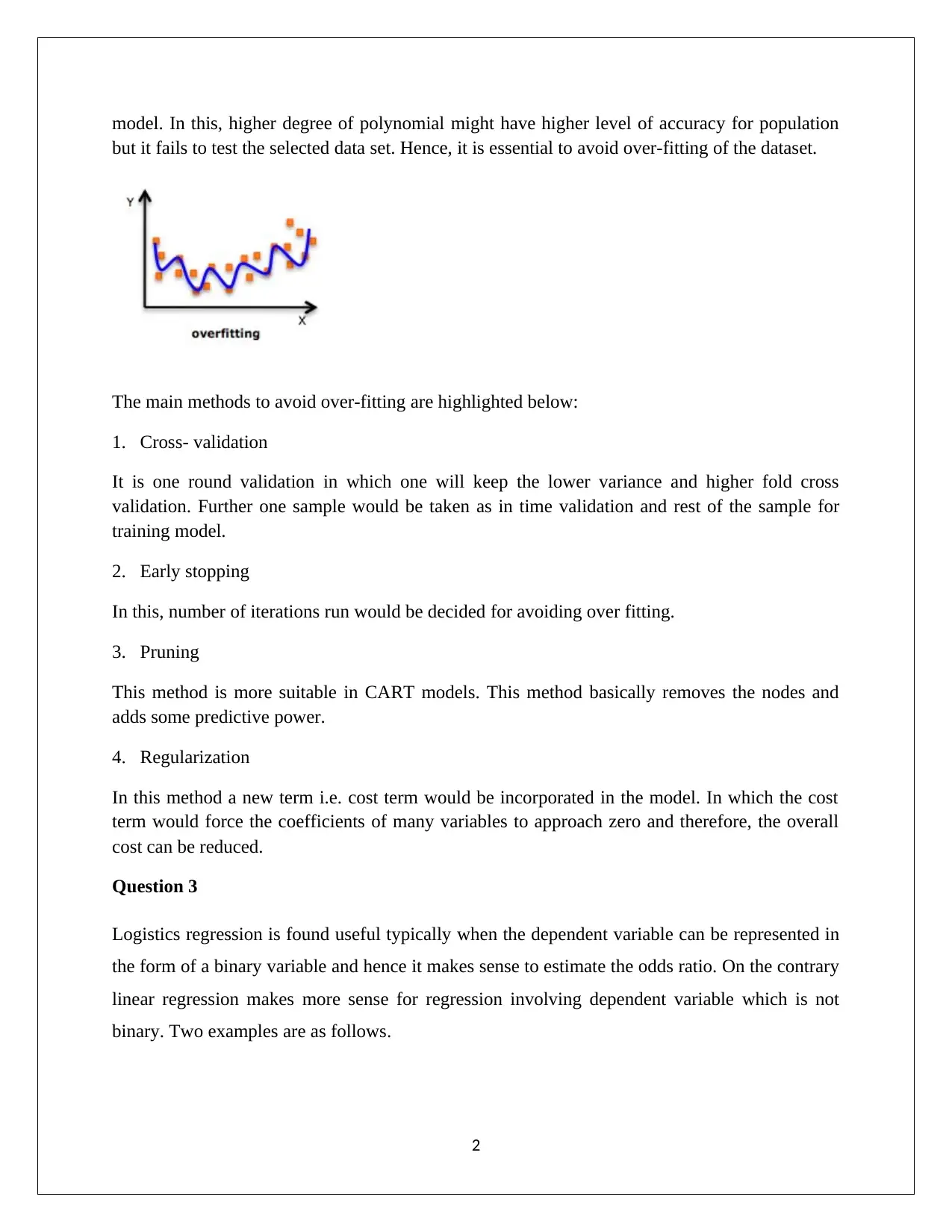
model. In this, higher degree of polynomial might have higher level of accuracy for population
but it fails to test the selected data set. Hence, it is essential to avoid over-fitting of the dataset.
The main methods to avoid over-fitting are highlighted below:
1. Cross- validation
It is one round validation in which one will keep the lower variance and higher fold cross
validation. Further one sample would be taken as in time validation and rest of the sample for
training model.
2. Early stopping
In this, number of iterations run would be decided for avoiding over fitting.
3. Pruning
This method is more suitable in CART models. This method basically removes the nodes and
adds some predictive power.
4. Regularization
In this method a new term i.e. cost term would be incorporated in the model. In which the cost
term would force the coefficients of many variables to approach zero and therefore, the overall
cost can be reduced.
Question 3
Logistics regression is found useful typically when the dependent variable can be represented in
the form of a binary variable and hence it makes sense to estimate the odds ratio. On the contrary
linear regression makes more sense for regression involving dependent variable which is not
binary. Two examples are as follows.
2

 One example which would require the use of logistic regression is with regards to
approval of loan by the new customers. In this particular case, there would be a binary
dependent variable as the loan may be approved or not. Thus, in such a case using a
linear regression would not serve the purpose as with varied set of independent variables,
it would not be possible to capture the output in binary form. As a result, it makes sense
to use logistic regression which can easily ensure this and thus would be appropriate.
 Another example would be in the context of passing or failing a particular exam based on
independent variables such as study time, presence on social media, lectures attended etc.
In this case also, the desired output would be captured as pass or fail and hence is binary
and therefore logistic regression would be preferred over linear regression. The logistic
regression would yield values between 0 and 1 which are essentially probability and
hence based on the same the odds of the two events can be computed. This is not the case
in linear regression which gives the absolute value of the dependent variable and not the
underlying probability.
SECTION B
Question 1
(a) The analyst found out 6 as the appropriate number of clusters by considering the output
shown in sheet 1-a-2-1 and also sheet 1-a-1-1 of the given output. The output in these two
selected sheets tends to highlight the output given when the data is based on 5 clusters
and 6 clusters respectively. The tables highlighting sum of square distances in cluster
need to be referred in both the sheets. It is apparent from cell D40 of sheet 1-a-1-1 that
the lowest intra cluster distance square is 3447.02 in case of five clusters. However, in
case of six clusters, this is lower as highlighted by cell D41 of sheet 1-a-2-1 giving a
value of 3188.82. Since the objective in clustering is to ensure that intra-cluster variation
is minimised, hence six clusters would be preferred over five clusters for the given data.
(b) The description of the six clusters by their average characteristics is carried out below.
 Cluster 1 (Married elderly customers) – High priced product (average price = $1,071) is
bought by the married elderly (greater than 55 years) who may or may not be members
and does not involve the use of discount cards. The average product category lies
between 2 and 3.
3

 Cluster 2 (Married middle age gender skewed customers) – High priced product (Average
price = $1,110) is bought on average by married customers aged 45-50 years having high
percentage of members and involves high usage of discount cards. Also, there is gender
skewing visible in this cluster. The average product category lies between 2 and 3.
 Cluster 3 (Unmarried young age customers)- High priced product (Average price =
$1,210) is bought on average by unmarried customers aged 33-35 years having low
percentage of members and involves average usage of discount cards. The average
product category lies between 2 and 3.
 Cluster 4 (Higher average product middle age customers): Low priced product (Average
price = $759) is bought dominantly by married customers aged 42-45 years having low
percentage of members and involves higher usage of discount cards. The average product
category is 4.
 Cluster 5 (Unmarried old customers) - High priced product (Average price = $1224) is
bought dominantly by unmarried customers with average age above 60 years having
higher percentage of members and involves lower than average usage of discount cards.
The average product category exceeds 4.
 Cluster 6 (Unmarried middle age customers) - Low priced product (Average price =
$743) is bought dominantly by unmarried customers (with high gender skewing) aged 40-
42 years having average representation of members and involves lower than average
usage of discount cards. The average product category lies between 3 and 4.
Question 2
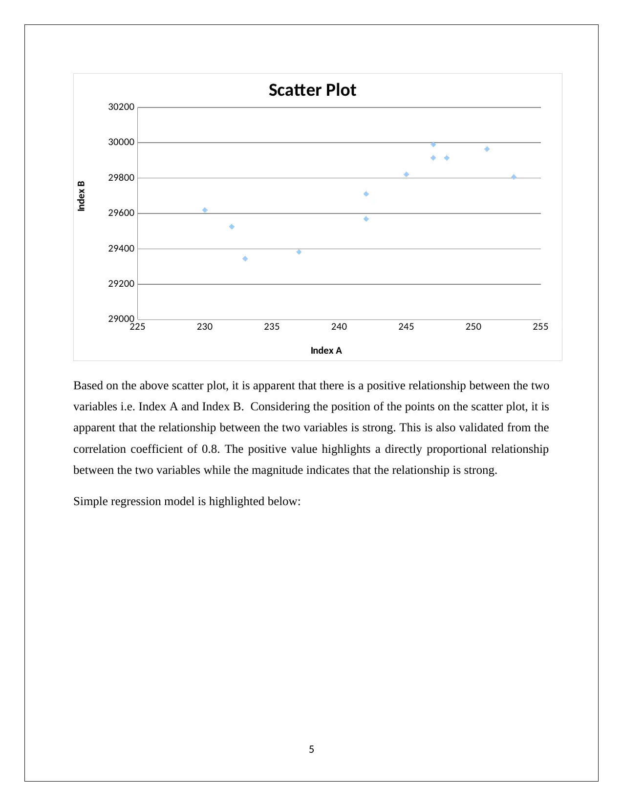
(a) The requisite scatter plot by taking index A as independent variable and index B as
dependent variable is highlighted below:
4

225 230 235 240 245 250 255
29000
29200
29400
29600
29800
30000
30200
Scatter Plot
Index A
Index B
Based on the above scatter plot, it is apparent that there is a positive relationship between the two
variables i.e. Index A and Index B. Considering the position of the points on the scatter plot, it is
apparent that the relationship between the two variables is strong. This is also validated from the
correlation coefficient of 0.8. The positive value highlights a directly proportional relationship
between the two variables while the magnitude indicates that the relationship is strong.
Simple regression model is highlighted below:
5

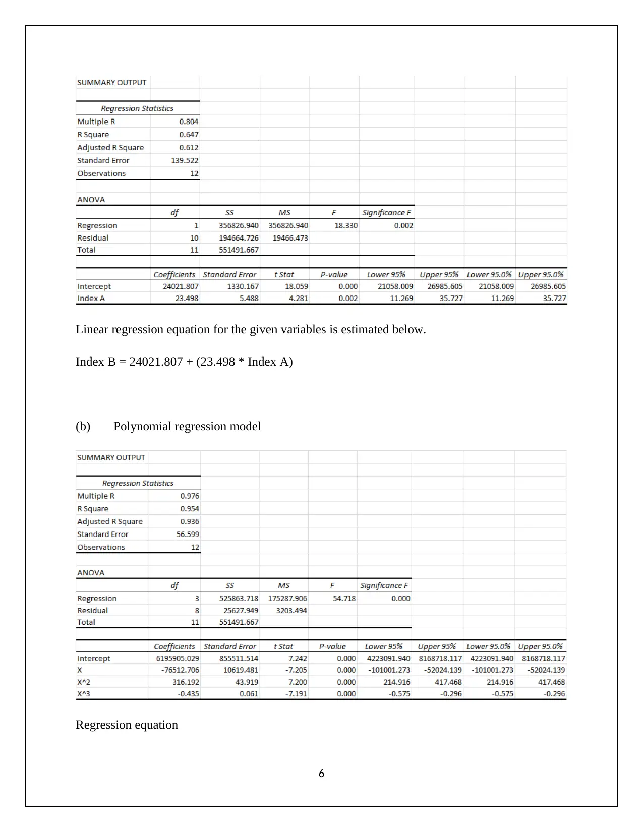
Linear regression equation for the given variables is estimated below.
Index B = 24021.807 + (23.498 * Index A)
(b) Polynomial regression model
Regression equation
6

Let
Index A = X
Index B = Y
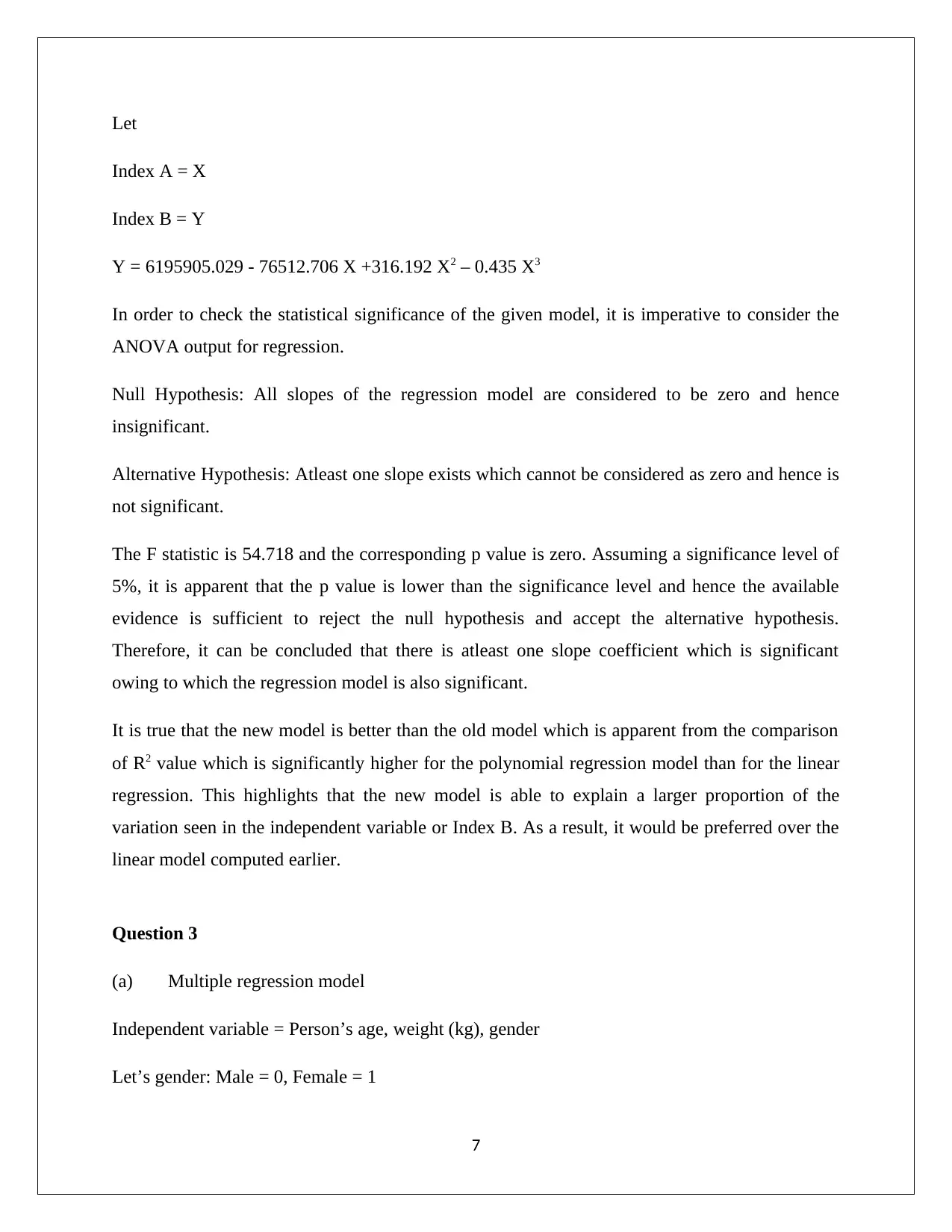
Y = 6195905.029 - 76512.706 X +316.192 X2 – 0.435 X3
In order to check the statistical significance of the given model, it is imperative to consider the
ANOVA output for regression.
Null Hypothesis: All slopes of the regression model are considered to be zero and hence
insignificant.
Alternative Hypothesis: Atleast one slope exists which cannot be considered as zero and hence is
not significant.
The F statistic is 54.718 and the corresponding p value is zero. Assuming a significance level of
5%, it is apparent that the p value is lower than the significance level and hence the available
evidence is sufficient to reject the null hypothesis and accept the alternative hypothesis.
Therefore, it can be concluded that there is atleast one slope coefficient which is significant
owing to which the regression model is also significant.
It is true that the new model is better than the old model which is apparent from the comparison
of R2 value which is significantly higher for the polynomial regression model than for the linear
regression. This highlights that the new model is able to explain a larger proportion of the
variation seen in the independent variable or Index B. As a result, it would be preferred over the
linear model computed earlier.
Question 3
(a) Multiple regression model
Independent variable = Person’s age, weight (kg), gender
Let’s gender: Male = 0, Female = 1
7

Dependent variable = Risk (%)
Regression equation
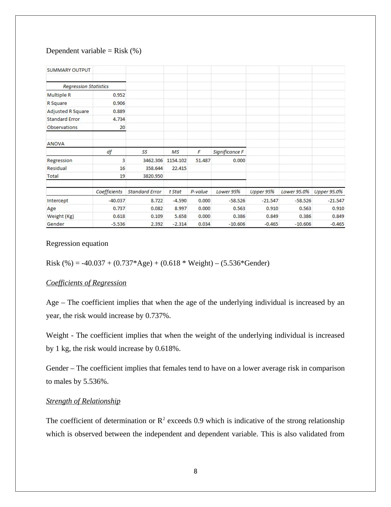
Risk (%) = -40.037 + (0.737*Age) + (0.618 * Weight) – (5.536*Gender)
Coefficients of Regression
Age – The coefficient implies that when the age of the underlying individual is increased by an
year, the risk would increase by 0.737%.
Weight - The coefficient implies that when the weight of the underlying individual is increased
by 1 kg, the risk would increase by 0.618%.
Gender – The coefficient implies that females tend to have on a lower average risk in comparison
to males by 5.536%.
Strength of Relationship
The coefficient of determination or R2 exceeds 0.9 which is indicative of the strong relationship
which is observed between the independent and dependent variable. This is also validated from
8

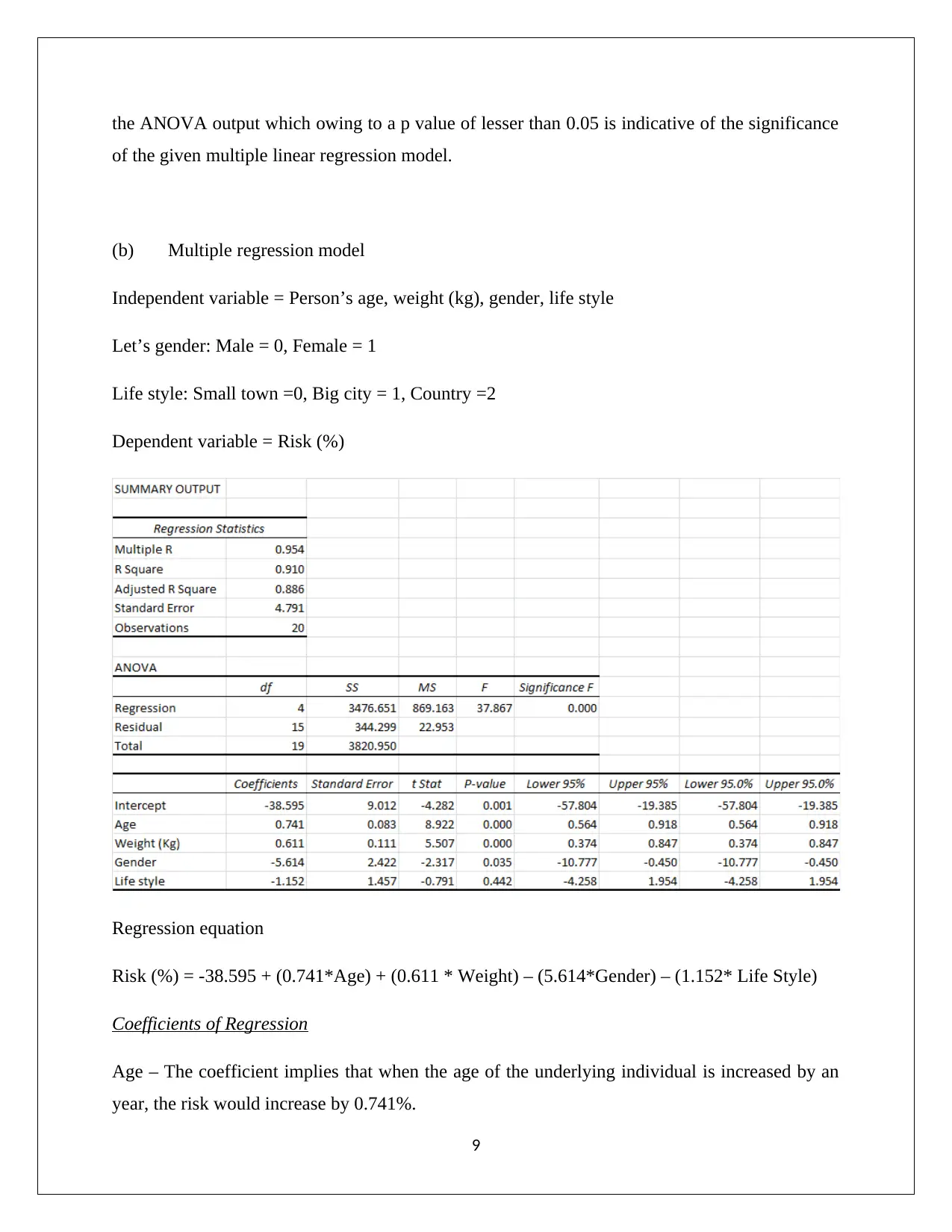
the ANOVA output which owing to a p value of lesser than 0.05 is indicative of the significance
of the given multiple linear regression model.
(b) Multiple regression model
Independent variable = Person’s age, weight (kg), gender, life style
Let’s gender: Male = 0, Female = 1
Life style: Small town =0, Big city = 1, Country =2
Dependent variable = Risk (%)
Regression equation
Risk (%) = -38.595 + (0.741*Age) + (0.611 * Weight) – (5.614*Gender) – (1.152* Life Style)
Coefficients of Regression
Age – The coefficient implies that when the age of the underlying individual is increased by an
year, the risk would increase by 0.741%.
9

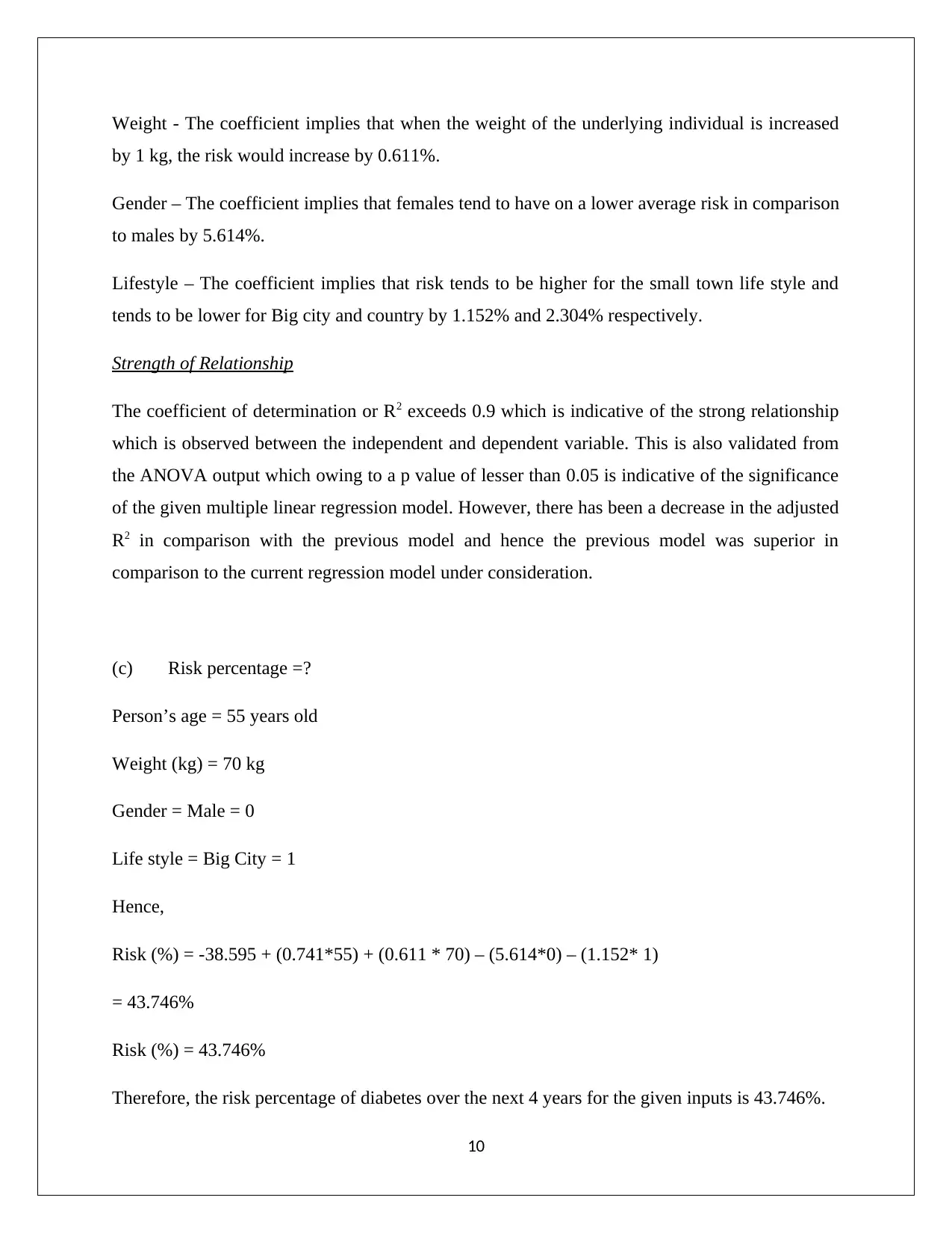
Weight - The coefficient implies that when the weight of the underlying individual is increased
by 1 kg, the risk would increase by 0.611%.
Gender – The coefficient implies that females tend to have on a lower average risk in comparison
to males by 5.614%.
Lifestyle – The coefficient implies that risk tends to be higher for the small town life style and
tends to be lower for Big city and country by 1.152% and 2.304% respectively.
Strength of Relationship
The coefficient of determination or R2 exceeds 0.9 which is indicative of the strong relationship
which is observed between the independent and dependent variable. This is also validated from
the ANOVA output which owing to a p value of lesser than 0.05 is indicative of the significance
of the given multiple linear regression model. However, there has been a decrease in the adjusted
R2 in comparison with the previous model and hence the previous model was superior in
comparison to the current regression model under consideration.
(c) Risk percentage =?
Person’s age = 55 years old
Weight (kg) = 70 kg
Gender = Male = 0
Life style = Big City = 1
Hence,
Risk (%) = -38.595 + (0.741*55) + (0.611 * 70) – (5.614*0) – (1.152* 1)
= 43.746%
Risk (%) = 43.746%
Therefore, the risk percentage of diabetes over the next 4 years for the given inputs is 43.746%.
10

Question 4
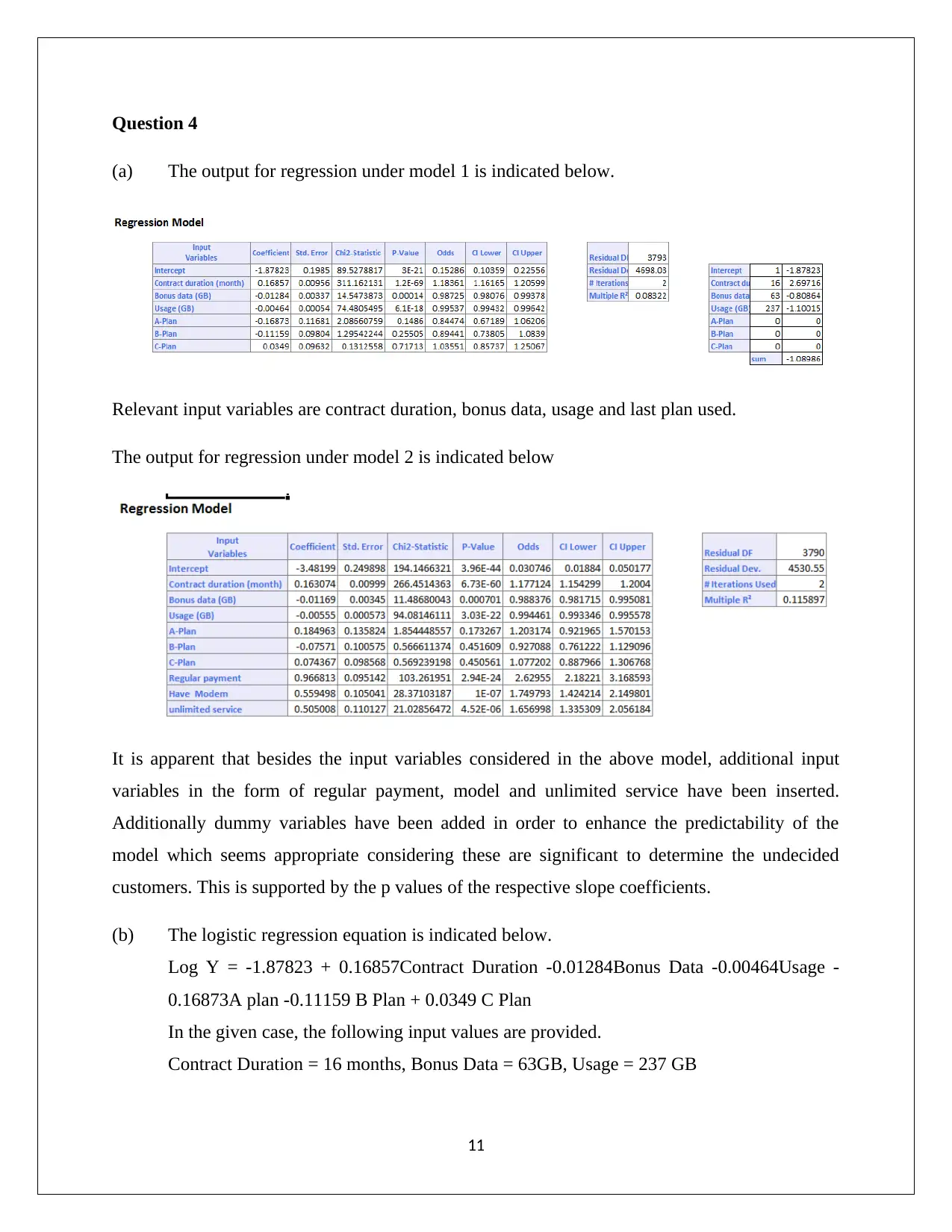
(a) The output for regression under model 1 is indicated below.
Relevant input variables are contract duration, bonus data, usage and last plan used.
The output for regression under model 2 is indicated below
It is apparent that besides the input variables considered in the above model, additional input
variables in the form of regular payment, model and unlimited service have been inserted.
Additionally dummy variables have been added in order to enhance the predictability of the
model which seems appropriate considering these are significant to determine the undecided
customers. This is supported by the p values of the respective slope coefficients.
(b) The logistic regression equation is indicated below.
Log Y = -1.87823 + 0.16857Contract Duration -0.01284Bonus Data -0.00464Usage -
0.16873A plan -0.11159 B Plan + 0.0349 C Plan
In the given case, the following input values are provided.
Contract Duration = 16 months, Bonus Data = 63GB, Usage = 237 GB
11

In case of plan A, Log Y = -1.87823 + 0.16857*16 -0.01284*63 -0.00464237-
0.16873*1= -1.25859
In case of plan B, Log Y = -1.87823 + 0.16857*16 -0.01284*63 -0.00464237-
0.11159*1= -1.20145
In case of plan C, Log Y = -1.87823 + 0.16857*16 -0.01284*63 -0.00464237+0.0349*1
= -1.05497
The average of the above three values would be the value of log Y to be considered since
in the absence of the precise data on the plan, there is an equal likelihood of the three
plans. Hence, log Y = -1.17167
Solving the above, we get Y = 0.067. This clearly highlights a high likelihood that the
considered person is not undecided.
(c) In the given case, the cutoff success probability is considered as 0.5. As a result, when the
predicted probability of success exceeds 0.5, it is classified under class 1 while
probability value of success lower than 0.5 results in class 0. Typically, the class 1 and
class 0 errors are based on the cutoff probability value. Errors would arise when the
predicted and actual values do not match. Hence for a case when the predicted value
comes out as 1 but the actual value if 0, there is an error. Based on this data, the
confusion matrix can also be derived which essentially indicates the actual cases where
there is matching and mismatching between the class 0 and class 1 cases based on the
actual and predicted values.
Class 0 errors % = (Total mismatch of 0 cases/ Total number of 0 cases)*100
Class 1 errors %= (Total mismatch of 1cases/ Total number of 1 cases)*100
The relevant output in case of validation data is indicated below.
12

In the context of the given data, a class 1 error is more undesirable since it would highlight a
person would be predicted as not undecided but actually this would be an undecided customer.
These are the customers who the company needs to actively identify and proactively approach to
enhance their market share.
(d) A higher accuracy would be expected for the model represented in sheet 4-2-1 in
comparison to the corresponding model highlighted in 4-1-1. This is apparent from the
fact that the additional input variables added for the model indicated in sheet 4-2-1 are all
significant which is apparent from the p values of their respective slope coefficients
owing to which the predicted value would be more accurate for this model. As a result,
the relative error would be lower for this model compared to the first model (indicated in
4-1-1).
Question 5
(a) Model to compute the profit for the European put option
The price of per put option is $1.5 and the exercise price is $29. Also, the price per share in eight
months is $26.4.
The profit can be determined with the help if IF function of excel which is shown below:
Normal View
13

Formula View
Therefore, the profit for the European put option would be $1.1.
(b) Data table to represent the profit per share for a share price in 8 months between $15 and
$35 per share with an increment of $1.
14

15