PID Controller Design and Comparison
VerifiedAdded on 2020/01/28
|53
|3958
|272
Project
AI Summary
This assignment focuses on designing a PID controller for a given system using two distinct methods: the Ziegler-Nichols process reaction method and the root locus method. Students will implement these designs in MATLAB, analyze their performance through step response plots, and compare the effectiveness of each approach. The assignment also involves plotting the root locus diagrams for both open-loop and closed-loop systems to visualize stability and performance characteristics.
Contribute Materials
Your contribution can guide someone’s learning journey. Share your
documents today.
Control and
Instrumentation
Instrumentation
Secure Best Marks with AI Grader
Need help grading? Try our AI Grader for instant feedback on your assignments.
PART A
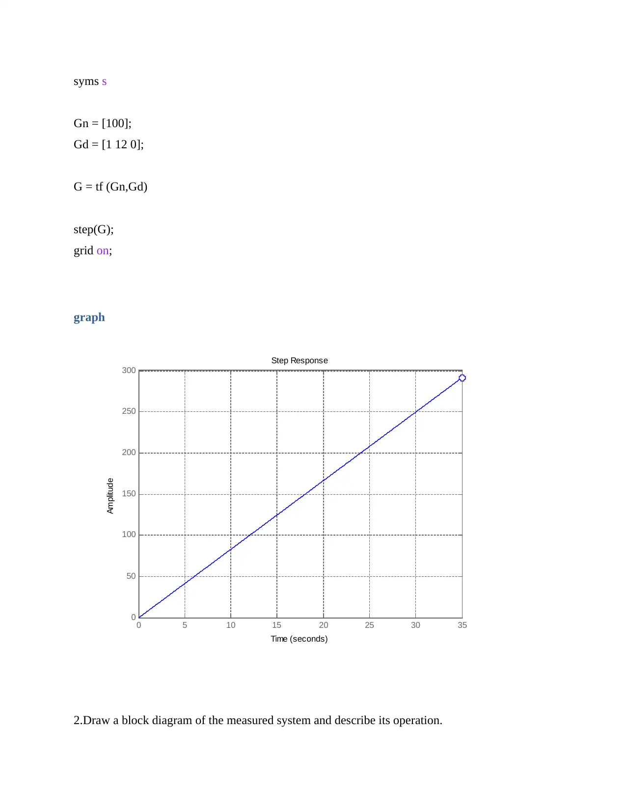
1.Obtain the step response timed output data from an instrument, linear and time invariant open
loop control system.
Sol: Linear and time invariant (LTI) system of 2nd order is as
T/F= C(S)/R(S)
= WO2/S2 + 2ƐWnS +Wn2 ( C.L.T.F)
T/F= C(S) / R(S) (O.L.T.F)
=WO2/S2 + 2ƐWnS
Let Wn=10 and Ɛ= 0.6
then, O.L.T.F will be
C(S)/R(S)= T/F = 102/S2 + 2 * 0.6 * 10
=100/S2 +12S
For step response r(t)=1 or R(s)= 1/s
so, C(S)= R(S)100/S2+12S
C(S)=1/S * 100/S2 +12S
C(S)= 100/S3 + 12S2
Matlab code
clear all;
clc;
syms s
Gn = [100];
Gd = [1 12 0];
G = tf (Gn,Gd)
step(G);
grid on;
graph
Step Response
Time (seconds)
Amplitude
0 5 10 15 20 25 30 35
0
50
100
150
200
250
300
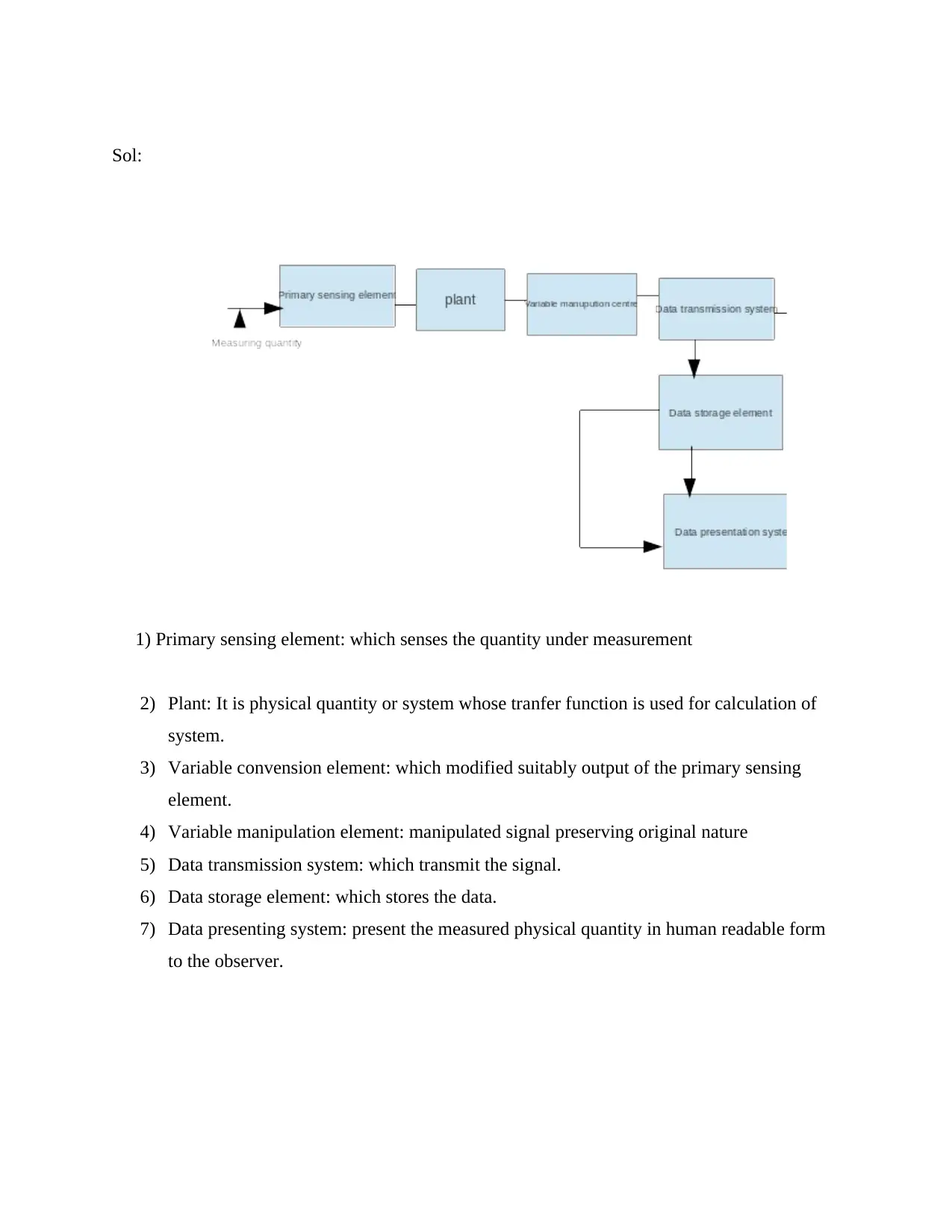
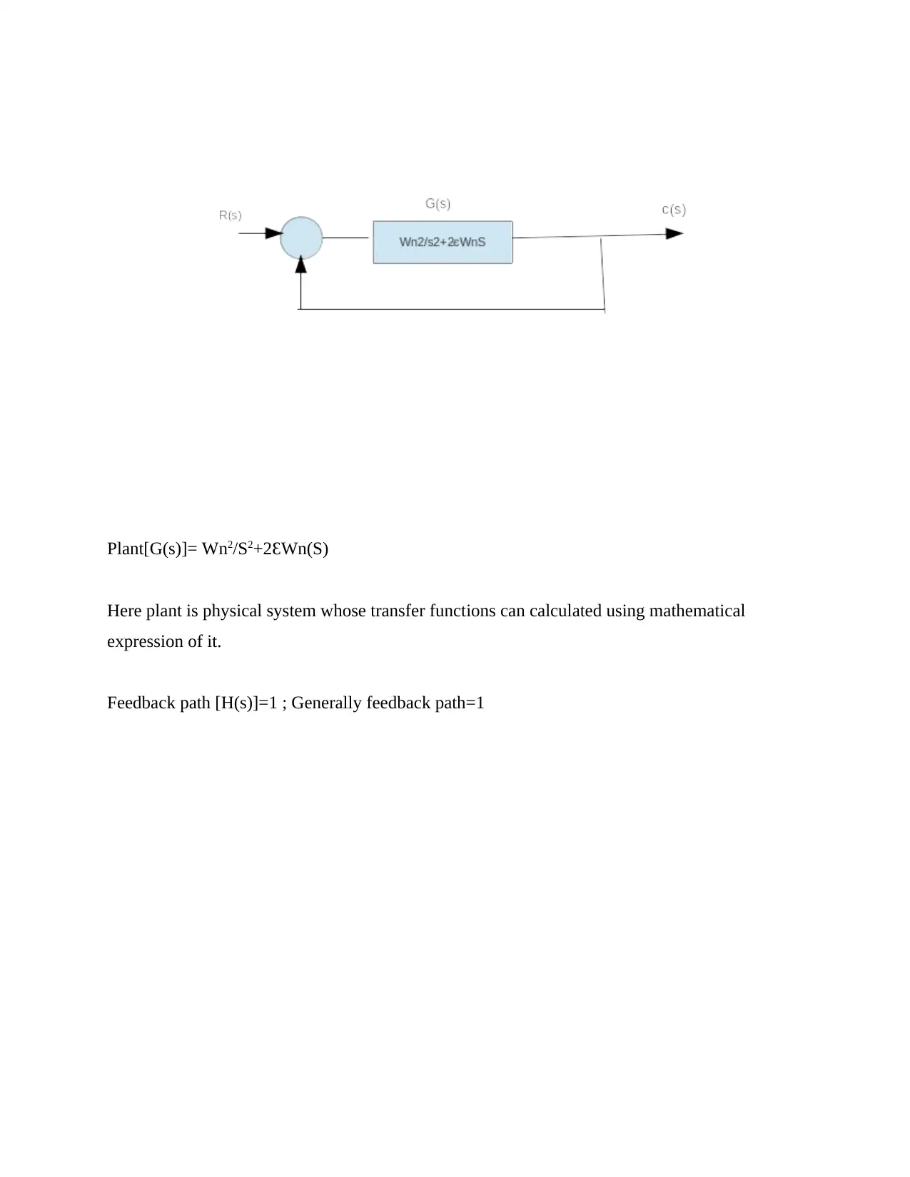
2.Draw a block diagram of the measured system and describe its operation.
Gn = [100];
Gd = [1 12 0];
G = tf (Gn,Gd)
step(G);
grid on;
graph
Step Response
Time (seconds)
Amplitude
0 5 10 15 20 25 30 35
0
50
100
150
200
250
300
2.Draw a block diagram of the measured system and describe its operation.
Sol:
1) Primary sensing element: which senses the quantity under measurement
2) Plant: It is physical quantity or system whose tranfer function is used for calculation of
system.
3) Variable convension element: which modified suitably output of the primary sensing
element.
4) Variable manipulation element: manipulated signal preserving original nature
5) Data transmission system: which transmit the signal.
6) Data storage element: which stores the data.
7) Data presenting system: present the measured physical quantity in human readable form
to the observer.
Secure Best Marks with AI Grader
Need help grading? Try our AI Grader for instant feedback on your assignments.
Plant[G(s)]= Wn2/S2+2ƐWn(S)
Here plant is physical system whose transfer functions can calculated using mathematical
expression of it.
Feedback path [H(s)]=1 ; Generally feedback path=1
Here plant is physical system whose transfer functions can calculated using mathematical
expression of it.
Feedback path [H(s)]=1 ; Generally feedback path=1
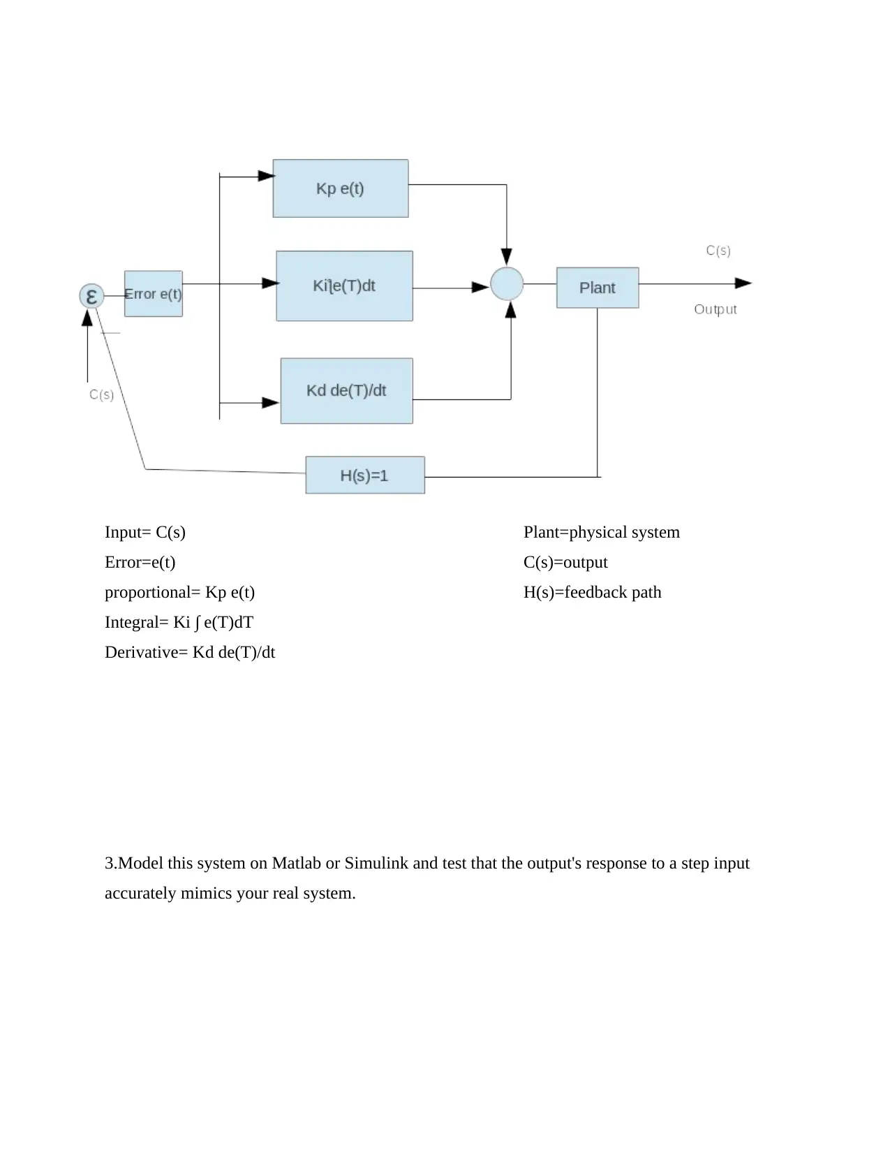
Input= C(s) Plant=physical system
Error=e(t) C(s)=output
proportional= Kp e(t) H(s)=feedback path
Integral= Ki ∫ e(T)dT
Derivative= Kd de(T)/dt
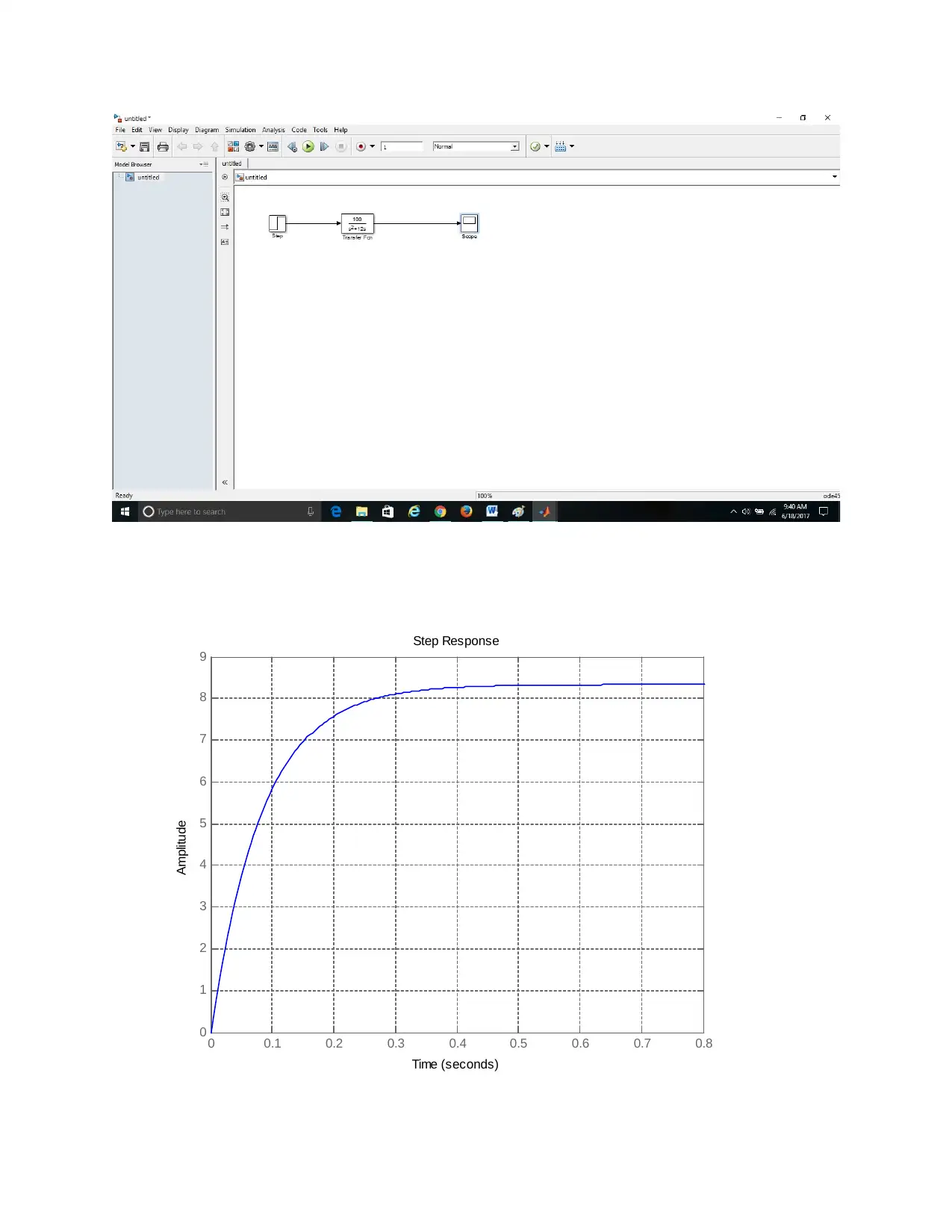
3.Model this system on Matlab or Simulink and test that the output's response to a step input
accurately mimics your real system.
Error=e(t) C(s)=output
proportional= Kp e(t) H(s)=feedback path
Integral= Ki ∫ e(T)dT
Derivative= Kd de(T)/dt
3.Model this system on Matlab or Simulink and test that the output's response to a step input
accurately mimics your real system.
0 0.1 0.2 0.3 0.4 0.5 0.6 0.7 0.8
0
1
2
3
4
5
6
7
8
9
Step Response
Time (seconds)
Amplitude
0
1
2
3
4
5
6
7
8
9
Step Response
Time (seconds)
Amplitude
Paraphrase This Document
Need a fresh take? Get an instant paraphrase of this document with our AI Paraphraser
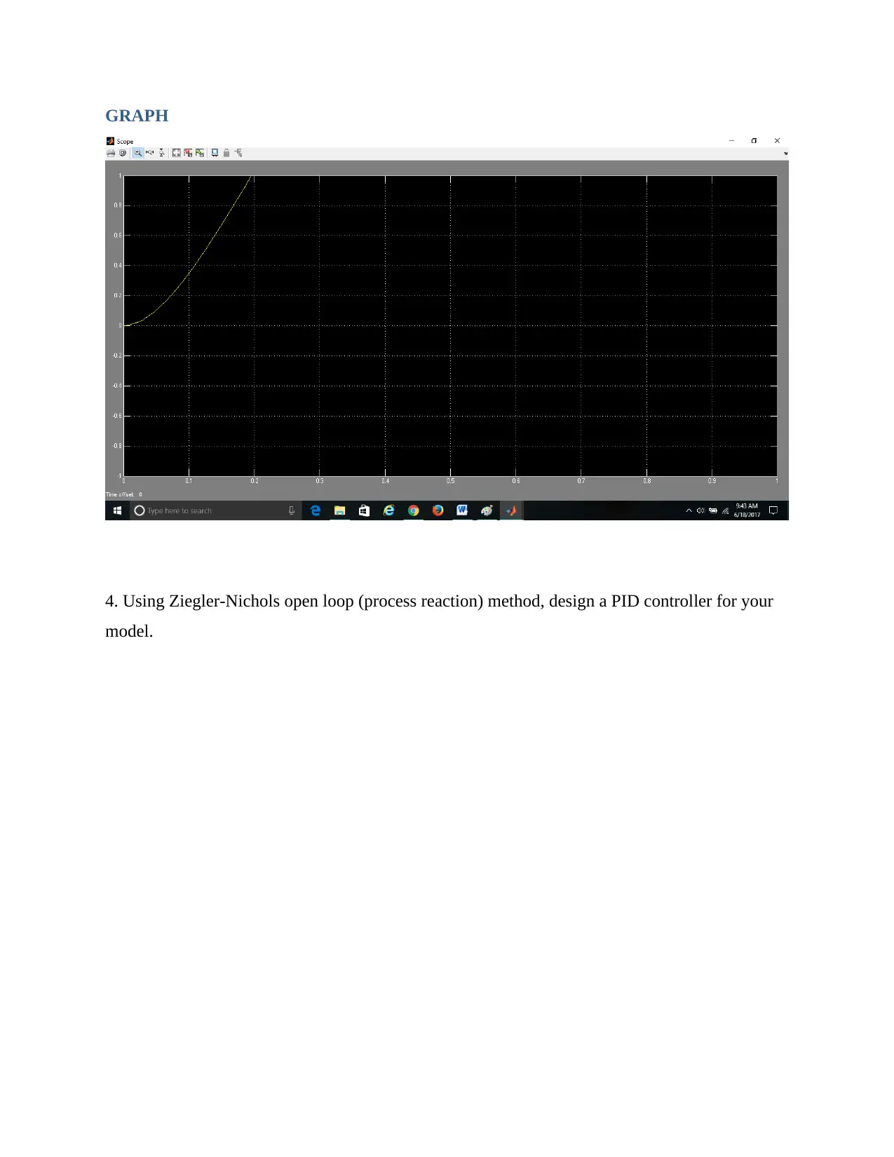
GRAPH
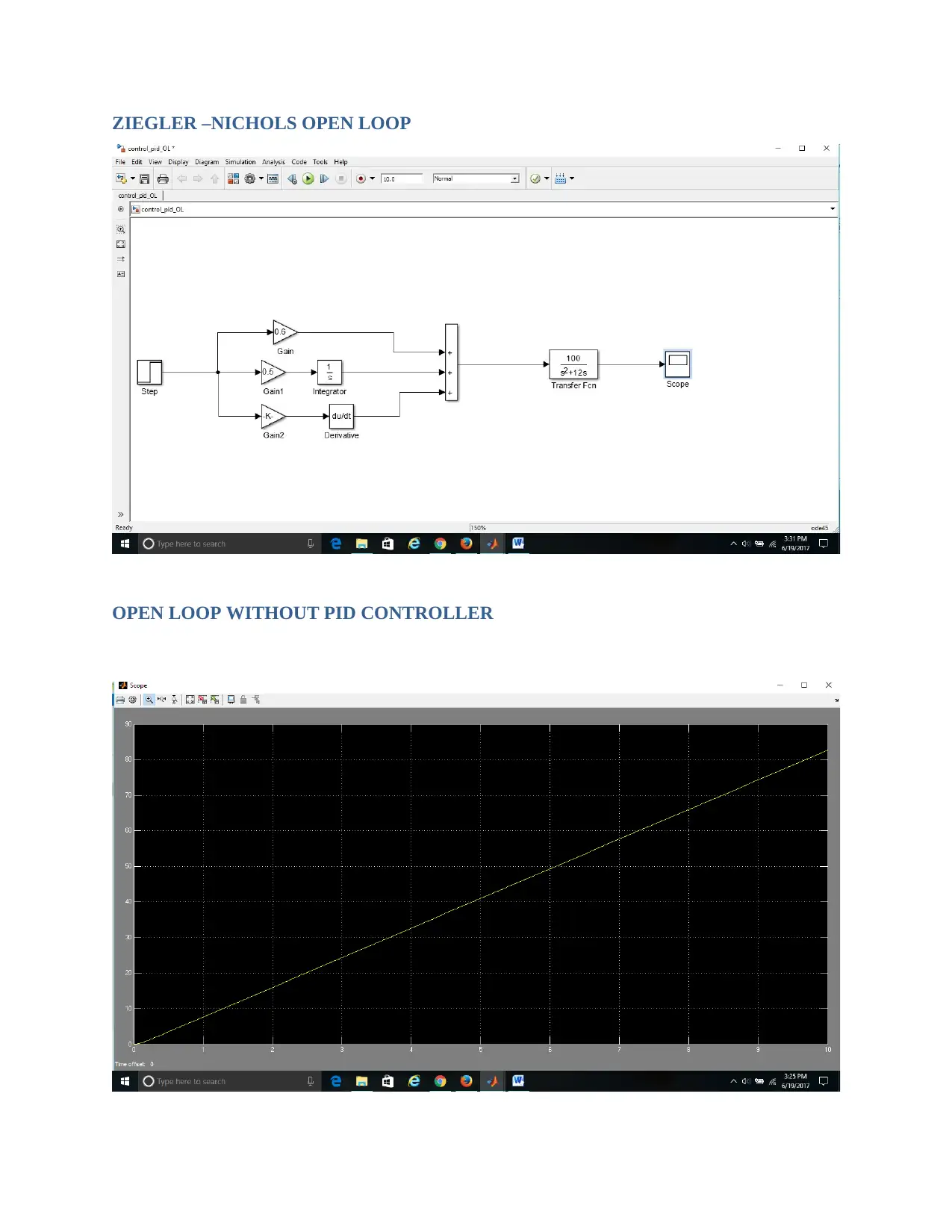
4. Using Ziegler-Nichols open loop (process reaction) method, design a PID controller for your
model.
4. Using Ziegler-Nichols open loop (process reaction) method, design a PID controller for your
model.
ZIEGLER –NICHOLS OPEN LOOP
OPEN LOOP WITHOUT PID CONTROLLER
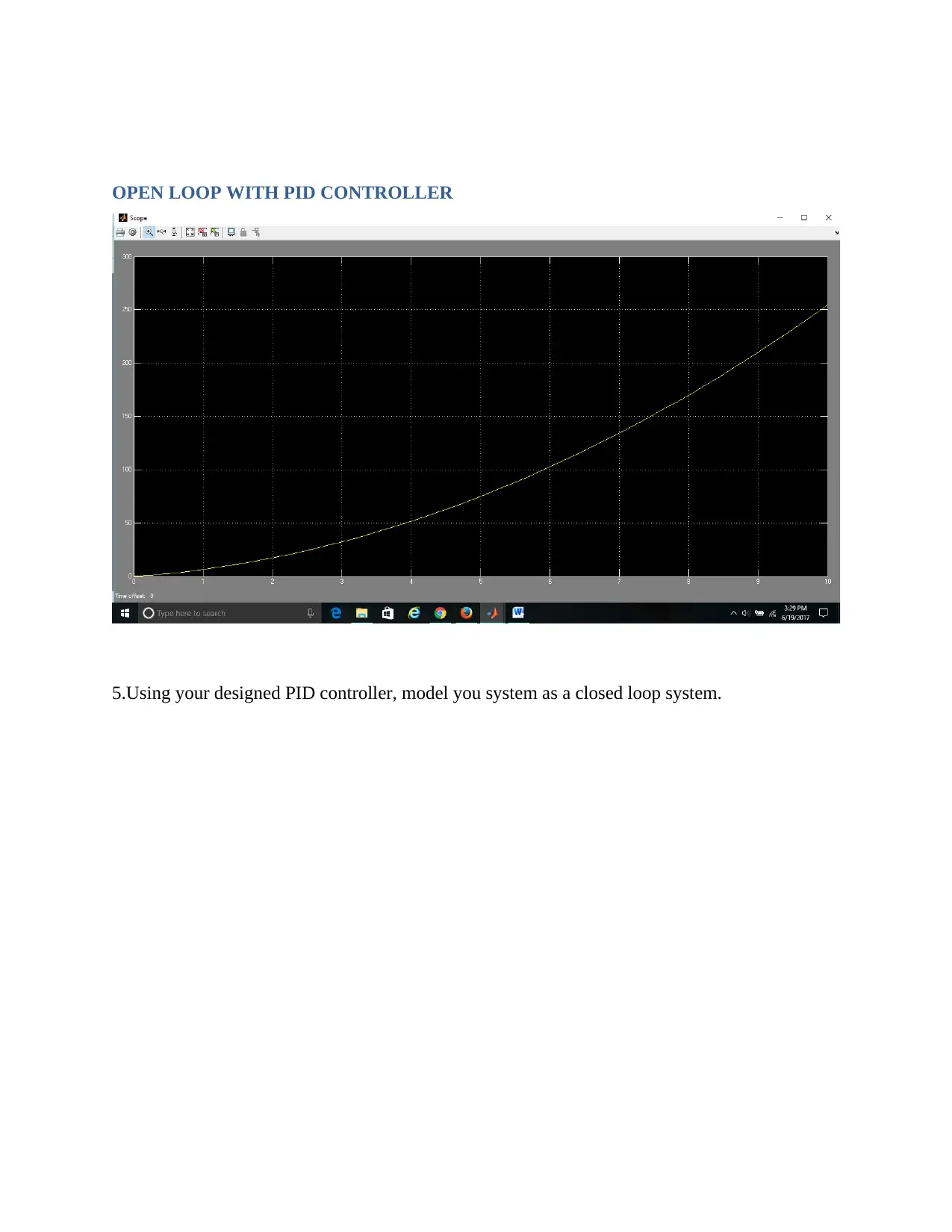
OPEN LOOP WITH PID CONTROLLER
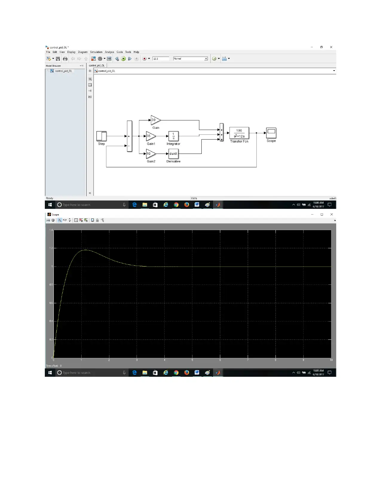
5.Using your designed PID controller, model you system as a closed loop system.
Secure Best Marks with AI Grader
Need help grading? Try our AI Grader for instant feedback on your assignments.
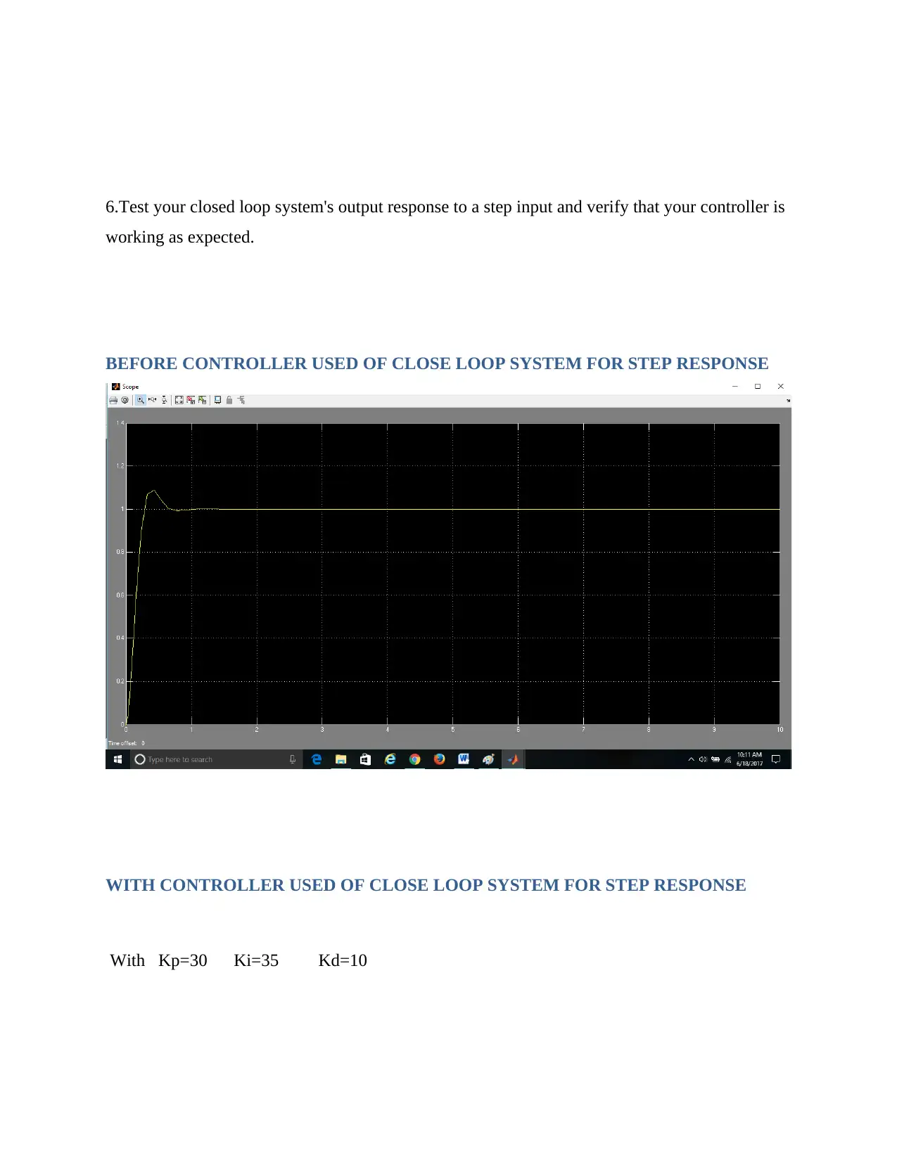
6.Test your closed loop system's output response to a step input and verify that your controller is
working as expected.
BEFORE CONTROLLER USED OF CLOSE LOOP SYSTEM FOR STEP RESPONSE
WITH CONTROLLER USED OF CLOSE LOOP SYSTEM FOR STEP RESPONSE
With Kp=30 Ki=35 Kd=10
working as expected.
BEFORE CONTROLLER USED OF CLOSE LOOP SYSTEM FOR STEP RESPONSE
WITH CONTROLLER USED OF CLOSE LOOP SYSTEM FOR STEP RESPONSE
With Kp=30 Ki=35 Kd=10
7.For the open loop system in Part(3), calculate the expected frequency response of this system,
considering low and high frequencies, poles, zeroes and dB frequency.
Paraphrase This Document
Need a fresh take? Get an instant paraphrase of this document with our AI Paraphraser
MATLAB CODE
clear all;
clc;
Z=0; % zero of system
P=[0,-12] % pole of system
K = 100; % gian of system
G = zpk(Z,P,K);
W =logspace(-3, 7, 1000000);
[MAG,PHASE] = bode(G,W);
PHASE = PHASE (1,:);
MAG = MAG(1,:);
PHASE_R = PHASE.*pi/180;
polar(PHASE_R,MAG) % polar plot(frequency response)
clear all;
clc;
Z=0; % zero of system
P=[0,-12] % pole of system
K = 100; % gian of system
G = zpk(Z,P,K);
W =logspace(-3, 7, 1000000);
[MAG,PHASE] = bode(G,W);
PHASE = PHASE (1,:);
MAG = MAG(1,:);
PHASE_R = PHASE.*pi/180;
polar(PHASE_R,MAG) % polar plot(frequency response)
GRAPH
2
4
6
8
10
30
210
60
240
90
270
120
300
150
330
180 0
8.Using the Simulink model of this open loop system, simulate the system to obtain output
frequency data in your preferred format(Nyquist plot, Bode plot or Nichols plot).
g =
100
----------
s^2 + 12 s
2
4
6
8
10
30
210
60
240
90
270
120
300
150
330
180 0
8.Using the Simulink model of this open loop system, simulate the system to obtain output
frequency data in your preferred format(Nyquist plot, Bode plot or Nichols plot).
g =
100
----------
s^2 + 12 s
Continuous-time transfer function.
BODE PLOT
-100
-50
0
50
Magnitude (dB)
10-1 100 101 102 103
-180
-135
-90
Phase (deg)
Bode Diagram
Frequency (rad/s)
NYQUIST PLOT
-1 -0.9 -0.8 -0.7 -0.6 -0.5 -0.4 -0.3 -0.2 -0.1 0
-15
-10
-5
0
5
10
15
0 dB
-10 dB-6 dB-4 dB
-2 dB
10 dB6 dB4 dB
2 dB
Nyquist Diagram
Real Axis
Imaginary Axis
BODE PLOT
-100
-50
0
50
Magnitude (dB)
10-1 100 101 102 103
-180
-135
-90
Phase (deg)
Bode Diagram
Frequency (rad/s)
NYQUIST PLOT
-1 -0.9 -0.8 -0.7 -0.6 -0.5 -0.4 -0.3 -0.2 -0.1 0
-15
-10
-5
0
5
10
15
0 dB
-10 dB-6 dB-4 dB
-2 dB
10 dB6 dB4 dB
2 dB
Nyquist Diagram
Real Axis
Imaginary Axis
Secure Best Marks with AI Grader
Need help grading? Try our AI Grader for instant feedback on your assignments.
9. Compare the Simulink frequency response results with your calculated results and critically
evaluate the accuracy of the model in terms of frequency response.
2
4
6
8
10
30
210
60
240
90
270
120
300
150
330
180 0
evaluate the accuracy of the model in terms of frequency response.
2
4
6
8
10
30
210
60
240
90
270
120
300
150
330
180 0
Given,open loop LTI Transfer function
G(S)=100/s2+12s
=Wn2/S2+2ƐWnS
=100/S(s+12)
Type 1 and order 2
G(jw)=100/-w2+j2w Ɵ=tan-1(-12/w)
G(jw)=100/(vo2)2 + (2w)2
Polar Plot
G(S)=100/s2+12s
=Wn2/S2+2ƐWnS
=100/S(s+12)
Type 1 and order 2
G(jw)=100/-w2+j2w Ɵ=tan-1(-12/w)
G(jw)=100/(vo2)2 + (2w)2
Polar Plot
Paraphrase This Document
Need a fresh take? Get an instant paraphrase of this document with our AI Paraphraser
PART B
clear all;
clc;
syms s
Gn = sym2poly( s+1);
Gd = sym2poly( s^3 + 19*s^2 + 100*s +150);
G = tf (Gn,Gd);
H = 1;
T = feedback (G,H);
clear all;
clc;
syms s
Gn = sym2poly( s+1);
Gd = sym2poly( s^3 + 19*s^2 + 100*s +150);
G = tf (Gn,Gd);
H = 1;
T = feedback (G,H);
step(T)
before PID control graph is as below
Step Response
Time (seconds)
Amplitude
0 0.5 1 1.5 2 2.5 3
0
0.002
0.004
0.006
0.008
0.01
0.012
System: T
Peak amplitude: 0.0103
Overshoot (%): 55.9
At time (seconds): 0.495
System: T
Settling time (seconds): 2.06 System: T
Final value: 0.00662
%%%%---------------------------my surname is DOLAN------------------------%%%%%%%
%%%%------------PID controller is design -----------------%%%%%%%%%%%%
Kp=811;
Ki=1000;
Kd=23;
G_controller = pid(Kp,Ki,Kd);
T_controller =feedback(G*G_controller,H);
step(T_controller);
grid on;
AFTER CONTROLLER PID USED
Step Response
Time (seconds)
Amplitude
0 0.5 1 1.5 2 2.5 3 3.5 4
0
0.2
0.4
0.6
0.8
1
1.2
1.4
System: T
Peak amplitude: 0.0103
Overshoot (%): 55.9
At time (seconds): 0.495
System: T_controller
Peak amplitude: 1.02
Overshoot (%): 2
At time (seconds): 0.102 System: T_controller
Final value: 1
System: T
Final value: 0.00662
T
T_controller
%%%%---------------------------my surname is DOLAN------------------------%%%%%%%
%%%------------------NORMAL TRANSFER FUNCTION AS GIVEN OPEN LOOP GAIN---%
%
Secure Best Marks with AI Grader
Need help grading? Try our AI Grader for instant feedback on your assignments.
clear all;
clc;
syms s
Gn = sym2poly( s+1);
Gd = sym2poly( s^3 + 20*s^2 + 105*s +155);
G = tf (Gn,Gd);
H = 1;
T = feedback (G,H);
step(T);
grid on;
hold on
%%%%------------PID controller is design -----------------%%%%%%%%%%%%
Kp=290;
Ki=1000;
Kd=2.5;
G_controller = pid(Kp,Ki,Kd);
T_controller =feedback(G*G_controller,H);
step(T_controller);
grid on;
MATLAB GRAPH PLOT
Step Response
Time (seconds)
Amplitude
0 0.5 1 1.5 2 2.5 3
0
0.2
0.4
0.6
0.8
1
1.2
1.4
System: T_controller
Peak amplitude: 1.05
Overshoot (%): 5.03
At time (seconds): 0.204
System: T
Peak amplitude: 0.00982
Overshoot (%): 53.2
At time (seconds): 0.5
System: T_controller
Final value: 1
System: T
Final value: 0.00641
T
T_controller
%%%%---------------------------my surname is DOLAN------------------------%%%%%%%
%%%------------------NORMAL TRANSFER FUNCTION AS GIVEN OPEN LOOP GAIN---%
%
clear all;
clc;
syms s
Gn = sym2poly( s+1);
Gd = sym2poly( s^3 + 20*s^2 + 110*s +160);
G = tf (Gn,Gd);
H = 1;
T = feedback (G,H);
step(T);
grid on;
hold on
%%%%------------PID controller is design -----------------%%%%%%%%%%%%
Kp=988;
Ki=1000;
Kd=17.4;
G_controller = pid(Kp,Ki,Kd);
T_controller =feedback(G*G_controller,H);
step(T_controller);
grid on;
Step Response
Time (seconds)
Amplitude
0 0.5 1 1.5 2 2.5 3 3.5 4 4.5
0
0.2
0.4
0.6
0.8
1
1.2
1.4
System: T
Peak amplitude: 0.00943
Overshoot (%): 51.8
At time (seconds): 0.481
System: T_controller
Peak amplitude: 1.08
Overshoot (%): 7.99
At time (seconds): 0.0937 System: T_controller
Final value: 1
System: T
Final value: 0.00621
T
T_controller
%%%%---------------------------my surname is DOLAN------------------------%%%%%%%
Paraphrase This Document
Need a fresh take? Get an instant paraphrase of this document with our AI Paraphraser
clear all;
clc;
syms s
Gn = sym2poly( s+1);
Gd = sym2poly( s^3 + 18*s^2 + 90*s +120);
G = tf (Gn,Gd);
H = 1;
T = feedback (G,H);
step(T);
grid on;
hold on
%%%%------------PID controller is design -----------------%%%%%%%%%%%%
Kp=180;
Ki=1000;
Kd=8.3;
G_controller = pid(Kp,Ki,Kd);
T_controller =feedback(G*G_controller,H);
step(T_controller);
grid on;
Step Response
Time (seconds)
Amplitude
0 1 2 3 4 5 6
0
0.2
0.4
0.6
0.8
1
1.2
1.4 System: T_controller
Peak amplitude: 1.02
Overshoot (%): 2.08
At time (seconds): 0.32
System: T
Time (seconds): 0.477
Amplitude: 0.0117
System: T_controller
Final value: 1
System: T
Final value: 0.00826
Time (seconds)
Amplitude
0 1 2 3 4 5 6
0
0.2
0.4
0.6
0.8
1
1.2
1.4 System: T_controller
Peak amplitude: 1.02
Overshoot (%): 2.08
At time (seconds): 0.32
System: T
Time (seconds): 0.477
Amplitude: 0.0117
System: T_controller
Final value: 1
System: T
Final value: 0.00826
%%%%---------------------------my surname is DOLAN------------------------%%%%%%%
clear all;
clc;
syms s
Gn = sym2poly( s+1);
Gd = sym2poly( s^3 + 18*s^2 + 85*s +100);
G = tf (Gn,Gd);
H = 1;
T = feedback (G,H);
step(T);
grid on;
hold on
%%%%------------PID controller is design -----------------%%%%%%%%%%%%
Kp=280;
Ki=1000;
Kd=9.4;
G_controller = pid(Kp,Ki,Kd);
clear all;
clc;
syms s
Gn = sym2poly( s+1);
Gd = sym2poly( s^3 + 18*s^2 + 85*s +100);
G = tf (Gn,Gd);
H = 1;
T = feedback (G,H);
step(T);
grid on;
hold on
%%%%------------PID controller is design -----------------%%%%%%%%%%%%
Kp=280;
Ki=1000;
Kd=9.4;
G_controller = pid(Kp,Ki,Kd);
Secure Best Marks with AI Grader
Need help grading? Try our AI Grader for instant feedback on your assignments.
T_controller =feedback(G*G_controller,H);
step(T_controller);
grid on;
Step Response
Time (seconds)
A m p lit u d e
0 0.5 1 1.5 2 2.5 3 3.5
0
0.2
0.4
0.6
0.8
1
1.2
1.4
System: T
Peak amplitude: 0.0129
Overshoot (%): 29.9
At time (seconds): 0.626
System: T_controller
Peak amplitude: 1.01
Overshoot (%): 1.12
At time (seconds): 0.222 System: T_controller
Final value: 1
System: T
Final value: 0.0099
%%%%---------------------------my surname is DOLAN------------------------%%%%%%%
clear all;
clc;
syms s
Gn = sym2poly( s+1);
Gd = sym2poly( s^3 + 20*s^2 + 105*s +120);
G = tf (Gn,Gd);
H = 1;
T = feedback (G,H);
step(T);
grid on;
hold on
%%%%------------PID controller is design -----------------%%%%%%%%%%%%
Kp=190;
Ki=1000;
Kd=5;
G_controller = pid(Kp,Ki,Kd);
T_controller =feedback(G*G_controller,H);
step(T_controller);
grid on;
G = tf (Gn,Gd);
H = 1;
T = feedback (G,H);
step(T);
grid on;
hold on
%%%%------------PID controller is design -----------------%%%%%%%%%%%%
Kp=190;
Ki=1000;
Kd=5;
G_controller = pid(Kp,Ki,Kd);
T_controller =feedback(G*G_controller,H);
step(T_controller);
grid on;
Step Response
Time (seconds)
Amplitude
0 0.5 1 1.5 2 2.5 3 3.5
0
0.2
0.4
0.6
0.8
1
1.2
1.4
System: T_controller
Final value: 1
System: T
Final value: 0.00826
System: T
Time (seconds): 0.543
Amplitude: 0.0104
System: T_controller
Peak amplitude: 1.02
Overshoot (%): 2.06
At time (seconds): 0.302
%%%%---------------------------my surname is DOLAN------------------------%%%%%%%
clear all;
clc;
syms s
Gn = sym2poly( s+1);
Gd = sym2poly( s^3 + 20*s^2 + 100*s +130);
G = tf (Gn,Gd);
H = 1;
T = feedback (G,H);
step(T);
grid on;
hold on
Paraphrase This Document
Need a fresh take? Get an instant paraphrase of this document with our AI Paraphraser
%%%%------------PID controller is design -----------------%%%%%%%%%%%%
Kp=410;
Ki=1000;
Kd=8.6;
G_controller = pid(Kp,Ki,Kd);
T_controller =feedback(G*G_controller,H);
step(T_controller);
grid on;
Step Response
Time (seconds)
Amplitude
0 0.5 1 1.5 2 2.5 3 3.5 4 4.5 5
0
0.2
0.4
0.6
0.8
1
1.2
1.4
System: T
Final value: 0.00763
System: T_controller
Final value: 1
System: T_controller
Peak amplitude: 1.01
Overshoot (%): 1.08
At time (seconds): 0.165
System: T
Peak amplitude: 0.0106
Overshoot (%): 38.8
At time (seconds): 0.559
2.Using the root locus method, as defined in Nise's Control system Engineering book(module
core book):Chapter 9, Example 9.5, design a closed loop system with PID controller, in Matlab
to achieve the specification in Table 1,specify to your surname 1st initial.
%%%%---------------------------my surname is DOLAN------------------------%%%%%%%
%%%------------------NORMAL TRANSFER FUNCTION AS GIVEN OPEN LOOP GAIN---%
%
clear all;
clc;
syms s
Gn = sym2poly( s+1);
Gd = sym2poly( s^3 + 19*s^2 + 100*s +150);
G = tf (Gn,Gd);
H = 1;
T = feedback (G,H);
rlocus(T);
grid on;
hold on
%%%%------------PID controller is design -----------------%%%%%%%%%%%%
Kp=811;
Ki=1000;
Kd=23;
G_controller = pid(Kp,Ki,Kd);
T_controller =feedback(G*G_controller,H);
rlocus(T_controller);
grid on;
H = 1;
T = feedback (G,H);
rlocus(T);
grid on;
hold on
%%%%------------PID controller is design -----------------%%%%%%%%%%%%
Kp=811;
Ki=1000;
Kd=23;
G_controller = pid(Kp,Ki,Kd);
T_controller =feedback(G*G_controller,H);
rlocus(T_controller);
grid on;
Secure Best Marks with AI Grader
Need help grading? Try our AI Grader for instant feedback on your assignments.
-120 -100 -80 -60 -40 -20 0 20
-30
-20
-10
0
10
20
30
0.890.940.97
0.988
0.997
0.350.640.80.890.940.97
0.988
0.997
20406080100120
0.350.640.8
Root Locus
Real Axis (seconds-1)
Imaginary Axis (seconds-1)
T
T_controller
%%%%---------------------------my surname is DOLAN------------------------%%%%%%%
%%%------------------NORMAL TRANSFER FUNCTION AS GIVEN OPEN LOOP GAIN---%
%
clear all;
clc;
syms s
Gn = sym2poly( s+1);
Gd = sym2poly( s^3 + 20*s^2 + 105*s +155);
G = tf (Gn,Gd);
H = 1;
T = feedback (G,H);
rlocus(T);
grid on;
hold on
%%%%------------PID controller is design -----------------%%%%%%%%%%%%
Kp=290;
Ki=1000;
Kd=2.5;
G_controller = pid(Kp,Ki,Kd);
T_controller =feedback(G*G_controller,H);
rlocus(T_controller);
grid on;
-400 -350 -300 -250 -200 -150 -100 -50 0 50
-150
-100
-50
0
50
100
150 0.870.93
0.97
0.992
0.240.460.640.780.870.93
0.97
0.992
50100150200250300350400
0.240.460.640.78
Root Locus
Real Axis (seconds-1
)
Imaginary Axis (seconds-1
)
T
T_controller
%%%%---------------------------my surname is DOLAN------------------------%%%%%%%
%%%------------------NORMAL TRANSFER FUNCTION AS GIVEN OPEN LOOP GAIN---%
%
clear all;
clc;
syms s
Gn = sym2poly( s+1);
Gd = sym2poly( s^3 + 20*s^2 + 110*s +160);
G = tf (Gn,Gd);
H = 1;
T = feedback (G,H);
rlocus(T);
grid on;
hold on
%%%%------------PID controller is design -----------------%%%%%%%%%%%%
Kp=988;
Ki=1000;
Kd=17.4;
G_controller = pid(Kp,Ki,Kd);
T_controller =feedback(G*G_controller,H);
rlocus(T_controller);
Paraphrase This Document
Need a fresh take? Get an instant paraphrase of this document with our AI Paraphraser
grid on;
-200 -150 -100 -50 0 50
-50
-40
-30
-20
-10
0
10
20
30
40
50 0.9450.974
0.99
0.997
0.40.660.820.90.9450.974
0.99
0.997
255075100125150175200
0.40.660.820.9
Root Locus
Real Axis (seconds-1
)
Imaginary Axis (seconds-1
)
T
T_controller
%%%%---------------------------my surname is DOLAN------------------------%%%%%%%
%%%------------------NORMAL TRANSFER FUNCTION AS GIVEN OPEN LOOP GAIN---%
%
clear all;
clc;
syms s
Gn = sym2poly( s+1);
Gd = sym2poly( s^3 + 18*s^2 + 90*s +120);
G = tf (Gn,Gd);
H = 1;
T = feedback (G,H);
rlocus(T);
grid on;
hold on
%%%%------------PID controller is design -----------------%%%%%%%%%%%%
Kp=180;
Ki=1000;
Kd=8.3;
G_controller = pid(Kp,Ki,Kd);
T_controller =feedback(G*G_controller,H);
rlocus(T_controller);
grid on;
H = 1;
T = feedback (G,H);
rlocus(T);
grid on;
hold on
%%%%------------PID controller is design -----------------%%%%%%%%%%%%
Kp=180;
Ki=1000;
Kd=8.3;
G_controller = pid(Kp,Ki,Kd);
T_controller =feedback(G*G_controller,H);
rlocus(T_controller);
grid on;
-35 -30 -25 -20 -15 -10 -5 0 5
-15
-10
-5
0
5
10
15 0.220.420.60.740.84
0.92
0.965
0.99
0.220.420.60.740.84
0.92
0.965
0.99
5101520253035
Root Locus
Real Axis (seconds-1
)
Imaginary Axis (seconds-1
)
T
T_controller
%%%%---------------------------my surname is DOLAN------------------------%%%%%%%
%%%------------------NORMAL TRANSFER FUNCTION AS GIVEN OPEN LOOP GAIN---%
%
clear all;
clc;
syms s
Gn = sym2poly( s+1);
Gd = sym2poly( s^3 + 18*s^2 + 85*s +100);
G = tf (Gn,Gd);
H = 1;
Secure Best Marks with AI Grader
Need help grading? Try our AI Grader for instant feedback on your assignments.
T = feedback (G,H);
rlocus(T);
grid on;
hold on
%%%%------------PID controller is design -----------------%%%%%%%%%%%%
Kp=280;
Ki=1000;
Kd=9.4;
G_controller = pid(Kp,Ki,Kd);
T_controller =feedback(G*G_controller,H);
rlocus(T_controller);
grid on;
rlocus(T);
grid on;
hold on
%%%%------------PID controller is design -----------------%%%%%%%%%%%%
Kp=280;
Ki=1000;
Kd=9.4;
G_controller = pid(Kp,Ki,Kd);
T_controller =feedback(G*G_controller,H);
rlocus(T_controller);
grid on;
-80 -70 -60 -50 -40 -30 -20 -10 0 10
-20
-15
-10
-5
0
5
10
15
20 0.9350.968
0.986
0.997
0.350.620.80.880.9350.968
0.986
0.997
1020304050607080
0.350.620.80.88
Root Locus
Real Axis (seconds-1
)
Imaginary Axis (seconds-1
)
T
T_controller
%%%%---------------------------my surname is DOLAN------------------------%%%%%%%
%%%------------------NORMAL TRANSFER FUNCTION AS GIVEN OPEN LOOP GAIN---%
%
clear all;
clc;
syms s
Gn = sym2poly( s+1);
Gd = sym2poly( s^3 + 20*s^2 + 105*s +120);
G = tf (Gn,Gd);
H = 1;
T = feedback (G,H);
rlocus(T);
grid on;
hold on
%%%%------------PID controller is design -----------------%%%%%%%%%%%%
Kp=190;
Ki=1000;
Kd=5;
G_controller = pid(Kp,Ki,Kd);
T_controller =feedback(G*G_controller,H);
rlocus(T_controller);
grid on;
Paraphrase This Document
Need a fresh take? Get an instant paraphrase of this document with our AI Paraphraser
-120 -100 -80 -60 -40 -20 0 20
-30
-20
-10
0
10
20
30 0.890.940.97
0.988
0.997
0.350.640.80.890.940.97
0.988
0.997
20406080100120
0.350.640.8
Root Locus
Real Axis (seconds-1
)
Imaginary Axis (seconds-1
)
T
T_controller
%%%%---------------------------my surname is DOLAN------------------------%%%%%%%
%%%------------------NORMAL TRANSFER FUNCTION AS GIVEN OPEN LOOP GAIN---%
%
clear all;
clc;
syms s
Gn = sym2poly( s+1);
Gd = sym2poly( s^3 + 20*s^2 + 100*s +130);
G = tf (Gn,Gd);
H = 1;
T = feedback (G,H);
rlocus(T);
grid on;
hold on
%%%%------------PID controller is design -----------------%%%%%%%%%%%%
Kp=410;
Ki=1000;
Kd=8.6;
G_controller = pid(Kp,Ki,Kd);
T_controller =feedback(G*G_controller,H);
rlocus(T_controller);
grid on;
H = 1;
T = feedback (G,H);
rlocus(T);
grid on;
hold on
%%%%------------PID controller is design -----------------%%%%%%%%%%%%
Kp=410;
Ki=1000;
Kd=8.6;
G_controller = pid(Kp,Ki,Kd);
T_controller =feedback(G*G_controller,H);
rlocus(T_controller);
grid on;
-160 -140 -120 -100 -80 -60 -40 -20 0 20
-40
-30
-20
-10
0
10
20
30
40 0.9350.968
0.986
0.997
0.350.620.80.880.9350.968
0.986
0.997
20406080100120140160
0.350.620.80.88
Root Locus
Real Axis (seconds-1
)
Imaginary Axis (seconds-1
)
T
T_controller
3.Test your closed loop system's output response to a step input and verify that your controller is
working as expected.
Secure Best Marks with AI Grader
Need help grading? Try our AI Grader for instant feedback on your assignments.
CLOSE LOOP OUTPUT RESPONSE TO A STEP RESPONSE
CLOSE LOOP OUTPUT RESPONSE TO A STEP RESPONSE WITH PID
CONTROLLER
CONTROLLER
4.Critically compare the two PID controller design methods: Ziegler Nicholas process reaction
versus root locus.
ZIEGLER NICHOL PID CONTROLLER
clc;
syms s
Gn = sym2poly( s+1);
Gd = sym2poly( s^3 + 19*s^2 + 100*s +150);
G = tf (Gn,Gd);
H = 1;
T = feedback (G,H);
step(T)
before PID control graph is as below
versus root locus.
ZIEGLER NICHOL PID CONTROLLER
clc;
syms s
Gn = sym2poly( s+1);
Gd = sym2poly( s^3 + 19*s^2 + 100*s +150);
G = tf (Gn,Gd);
H = 1;
T = feedback (G,H);
step(T)
before PID control graph is as below
Paraphrase This Document
Need a fresh take? Get an instant paraphrase of this document with our AI Paraphraser
Step Response
Time (seconds)
Amplitude
0 0.5 1 1.5 2 2.5 3
0
0.002
0.004
0.006
0.008
0.01
0.012
System: T
Peak amplitude: 0.0103
Overshoot (%): 55.9
At time (seconds): 0.495
System: T
Settling time (seconds): 2.06 System: T
Final value: 0.00662
%%%%---------------------------my surname is DOLAN------------------------%%%%%%%
%%%%------------PID controller is design -----------------%%%%%%%%%%%%
Kp=811;
Ki=1000;
Kd=23;
G_controller = pid(Kp,Ki,Kd);
T_controller =feedback(G*G_controller,H);
step(T_controller);
grid on;
AFTER CONTROLLER PID USED
Step Response
Time (seconds)
Amplitude
0 0.5 1 1.5 2 2.5 3 3.5 4
0
0.2
0.4
0.6
0.8
1
1.2
1.4
System: T
Peak amplitude: 0.0103
Overshoot (%): 55.9
At time (seconds): 0.495
System: T_controller
Peak amplitude: 1.02
Overshoot (%): 2
At time (seconds): 0.102 System: T_controller
Final value: 1
System: T
Final value: 0.00662
T
T_controller
ROOT LOCUS PID CONTOLLER
%%%%---------------------------my surname is DOLAN------------------------%%%%%%%
%%%------------------NORMAL TRANSFER FUNCTION AS GIVEN OPEN LOOP GAIN---%
%
clear all;
clc;
syms s
Gn = sym2poly( s+1);
Gd = sym2poly( s^3 + 19*s^2 + 100*s +150);
G = tf (Gn,Gd);
H = 1;
T = feedback (G,H);
rlocus(T);
grid on;
hold on
%%%%------------PID controller is design -----------------%%%%%%%%%%%%
Kp=811;
Ki=1000;
Kd=23;
G_controller = pid(Kp,Ki,Kd);
T_controller =feedback(G*G_controller,H);
rlocus(T_controller);
grid on;
Secure Best Marks with AI Grader
Need help grading? Try our AI Grader for instant feedback on your assignments.
-120 -100 -80 -60 -40 -20 0 20
-30
-20
-10
0
10
20
30
0.890.940.97
0.988
0.997
0.350.640.80.890.940.97
0.988
0.997
20406080100120
0.350.640.8
Root Locus
Real Axis (seconds-1)
Imaginary Axis (seconds-1)
T
T_controller
-30
-20
-10
0
10
20
30
0.890.940.97
0.988
0.997
0.350.640.80.890.940.97
0.988
0.997
20406080100120
0.350.640.8
Root Locus
Real Axis (seconds-1)
Imaginary Axis (seconds-1)
T
T_controller
1 out of 53
Related Documents
Your All-in-One AI-Powered Toolkit for Academic Success.
+13062052269
info@desklib.com
Available 24*7 on WhatsApp / Email
Unlock your academic potential
© 2024 | Zucol Services PVT LTD | All rights reserved.