PGBM 142 - Risk Management, Diversification, and Investment Appraisal
VerifiedAdded on 2023/06/16
|16
|4528
|426
Report
AI Summary
This report delves into corporate financial management, focusing on risk mitigation through diversification and various investment appraisal techniques. It begins by explaining how businesses balance profit maximization with risk minimization, emphasizing diversification as a strategy to reduce unpredictability. The report then evaluates Sporty PLC using P/E ratio, dividend valuation approach, and discounted cash flow (DCF) analysis to determine its value for a potential acquisition by RR Ltd. The DCF analysis projects future cash flows to assess the investment's feasibility. Finally, the report discusses a project by RR LTD, employing Net Present Value (NPV) to evaluate investment opportunities in Wolverhampton, considering different probabilities and potential returns. Desklib offers this and many other solved assignments for students.

PGBM 142 Corporate
financial management
financial management
Paraphrase This Document
Need a fresh take? Get an instant paraphrase of this document with our AI Paraphraser

Contents
Contents...........................................................................................................................................2
INTRODUCTION...........................................................................................................................3
PART B...........................................................................................................................................3
Task 1...........................................................................................................................................3
Task 2...........................................................................................................................................3
Task 3...........................................................................................................................................6
CONCLUSION................................................................................................................................1
REFERENCES................................................................................................................................2
INTRODUCTION
Every stakeholder strives to maximise profits whilst minimising risk. Every function
includes a threat which is compensated by a return (Alziyadat and Ahmed, 2019). The bigger the
risk, the higher the gain, as the saying goes. As a consequence, in attempt to maximise earnings,
a purchaser should accept more threats. Broadening your portfolio among many items with
different rewards and disadvantages is another way to reduce unpredictability. The first half of
this study examines how a business person could manage threat and profitability. Several
techniques to evaluating a company are discussed in the following report. For a better
understanding, the study's concluding portion illustrates investment assessment approaches.
PART B
Task 1
Diversification is a risk-mitigation strategy wherein a fund's or commodity's interests are
varied. Pension scheme diversification refers to participating in multi-asset approaches that give
members with elevated risk-adjusted returns. Private pensions participate in different securities
to stabilize the market and increase predicted returns. The objective of this essay is to show how
variety decreases risk whilst raising future earnings. The goal of diversification in private
pensions is to reduce risks such as economic and funding choices. Variability in the business
occurs as a consequence of factor influencing an entire market sector, such as borrowing costs
and currencies prices (Aureli, Magnaghi and Salvatori, 2019). Investment instability occurs when
such an individual firm's earnings miss the mark. In various pension plans, risks are spread
among a variety of product kinds. Moreover, a diversification plan decreases the downside risk
which might occur when pension money is engaged in a particular type of endeavour. Coefficient
values may aid in increasing investment variety. Connectivity is utilised in investing
management to look at a situation comprised of stocks in the plan. A statistically significant
correlation means that assets are travelling in the same direction, whilst a weak relationship
means that assets are going the opposite way. As an outcome, low-correlation assets are put
together to create diversification. The unpredictability of the content of information of assets is
reduced as capital is invested in multiple directions.
Members in the CAPM model have a wide range of financial classifications, which helps
to reduce overall instability. As a consequence, rather than a general hazard, the relevant risk is a
repeating concern. As a reason, employees that undertake deliberate chances rather than
opportunity cost might expect higher profits.
Task 2
Sporty PLC is being acquired by the management of RR Ltd. Sporty PLC, on either side,
has failed amid the establishment of a men's apparel business. As per CEOs polled, the reduction
⊘ This is a preview!⊘
Do you want full access?
Subscribe today to unlock all pages.

Trusted by 1+ million students worldwide
is attributable to an inability to predict current tastes and tendencies. Before proceeding with the
acquisition, RR Ltd should initially determine the value of Sporty Ltd (Chaston, 2017). As a
consequence, the purpose of this task is to determine Sporty Ltd's value utilizing the P/E ratio,
payout evaluation technique, and DCF research, as detailed below-
P/E ratio-
The price/earnings ratio is calculated by dividing the fair value of the present component
value of units by the company's income each piece. Using the P/E ratio, one could establish if
RR Ltd overvalued or undervalued the sporty PLC shares. The EPS of Sporty PLC is calculated
by splitting net profit after taxation by the number of units authorized.
EPS = net profit/number of shares outstanding Net profit = £4200000
Weighted average dividend = 9 / 100 * Sale (£ 20 m)
= 9 / 100 * £ 20 m
=0.09 * $ 20000000
= $ 1800000
Number of shares £1 = I shares
£40000000 = ? shares (£40000000 * 1 share )/£1
= £40000000 / £1
= 40000000 shares
EPS = 4200000 / 40000000 =0.105
This implies that one item of sporty is equivalent £0.105 in stock, showing that the
market value of a corporation is conservatively calculated. As a consequence, the firm would
profit £0.105 each piece from its current inventory (Chen, Tan and Fang, 2018). The price-to-
earnings ratio would've been 9.523 (1/£0.105).
Dividend Valuation Approach-
It is used to estimate the industry's value as the present value of all expected future
dividends payments. As shown below, the stock value is calculated by multiplied the payouts
each piece by the required bond yields less the payout productivity increase.
Stock value = dividend per share / ( required rate of return – dividend growth rate )
= 9 / ( 17 % - 9 % )
= 9 / ( 8 % )
= 9 / ( 0.08 )
= £112.5 m
To calculate the percentages of interest, divide the dividends distribution by the shares
valuation and multiplied by the annual productivity increase. The stock price is calculated by
multiplied the stock payment amount by the total revenue.
Rate of return = (dividend payment/stock price) + dividend growth rate
Stock price = £6 ( 9 % -7 % )
Paraphrase This Document
Need a fresh take? Get an instant paraphrase of this document with our AI Paraphraser
= £6 ( 2 % )
= £6 * 2 / 100.
= £6 * 0.02
Calculation of Discounted Cash Flow Value-
It approach is a strategically investment tool that determines the value of a company
based on projected future capital inflows. In terms of discounting cash flow, the company
employs a method similar to NPV (Cuong and Nhung, 2017). DCF, on either side, gauges a
program's present and future value. The DCF model supports investors in their judgement call
processes. Businesses should continue to invest in ventures that would be in high growth in the
future. This strategy often assumes that cash flows will be spread out over similar periods of time
and also that annual discounting levels will be used. RR Ltd will decide how to distribute its $ 20
billion in income that will be placed at an annual return income of 12%. The DCF starts by
estimating the anticipated cash flow. We might compute earning prospective using the 4%
annual increase depending on RR LTD's attributable earnings in year 1. Following that, the
approach replicates the present value of potential gains. The company expense under the DCF
technique is the present value of expected earnings. The enterprise is practicable if the financial
value of the project surpasses the initial expenditure that really is, if the sum of the cumulative
valuation of cash flow surpasses the initial expenditure. If the company's value surpasses the
initial investment, it is considered profitable. Investors, on either side, will usually participate in
projects with a high corporate value because these are highly lucrative. As a consequence, Sporty
PLC's company assessment according to the DCF method is as described in the following:
Year 1 2 3 4 5
Distributable
earnings
£4.2M £4.368M £4.543M £4.724M £4.913M
PVIF @12% 0.8929 0.7972 0.7118 0.6355 0.5674
PV of distributable
earnings
£3.7018M £3.4822M £3.2337M £3.0021M £2.7876M
The total present value of available for distribution earnings is £16.2074M. Since the
initial cost was £12 million, the stock's present value is 16.2074M - 20M= -£3.7926M. A project
with a negative present worth is doomed to fail and should be ignored (Fan and Chatterjee,
2018).
Description of Sporty's Value and Acquisition Prospects-
Sporty's stock prices were £750.6 million, but the buying prices were expected to be
£112.5 million. Because this shares value is higher than the expected shares value, Sporty PLC's
stock is overvalued. An inflating stock industry has been growing at a far faster pace than the
company's earnings or profits. If the balanced divide is higher, the annual dividend yields will
generate more income after purchase. Since the current stake is selling at a trade price of 60%,
RR ltd will benefit greatly from replicating profits during the acquisition of sporty. RR Ltd opted
lateral acquisition since it will provide greater income and equalize the shareholder wealth, thus
it is suggested to acquire sporty. Sporty PLC is unproductive in terms of forecasted future flow
since its net present value is negative. This signifies that the investment return is less than the
initial expenditure. Sporty Ltd's value in terms of price per profits ratio, Asset Price Principle,
and Discounted Working Capital Method justify the longitudinal buy. Sporty Plc should operate
as a competitive differentiator owing to its insufficient revenue. Sporty PLC's stocks are
overvalued, so the two companies cannot merge. Before purchasing Sporty Ltd, RR Ltd must
consider profits, shareholders wealth, annual levels of profitability, and the number of items
available (Idris, Krishnan and Azmi, 2017).
Task 3
The founders of RR LTD decided to design and produce in-house in Wolverhampton.
Opportunities for expansion in Asian nations would've been promising, but they'd be mitigated
by the fact that the business would've been located in Vietnamese. The following is a summary
of RR Ltd's information:
Year 1
The initial expenditure is projected to be £20 million, with a 0.55 chance of yielding £1.7
million in year one. With a chance of 0.45, you'll win £1 million.
Year 2
Considering the present market value of £1.7 million, the return in year 2 could be £2.8
million with a probability of 0.6 or £1.9 million with a probability of 0.4. If you make £1 million
in year one, you have a potential of receiving £1.1 million with a probability of 0.5 or £600,000
with a probability of 0.5 in year two. The projected revenue inflow percentage is anticipated to
be 5%.
During the first year
Invest £20 million with a return of £1.7 million, a decline, with a potential of 0.55. Year 2
is the project's next year.
Return £2.8 m with a probability of 0.6
If this results in $ 1.9 m with a probability of 0.4
£1m with the probability of 0.5 in the year 1
£600000 with a probability of 0.5 in the year 2
NPV that is presumed-
The repayment time is being used in the NPV technique of appraisal to assess firms and
investments. It is the sum of all net present value method. The required return levels are widely
⊘ This is a preview!⊘
Do you want full access?
Subscribe today to unlock all pages.

Trusted by 1+ million students worldwide
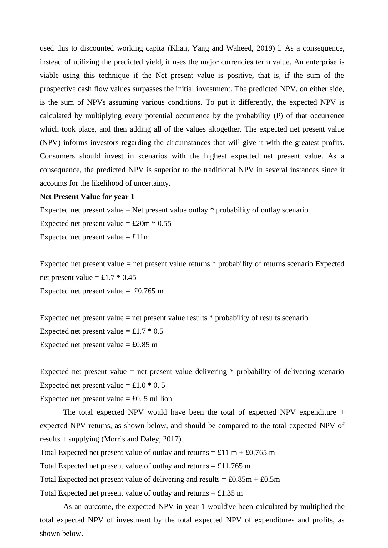
used this to discounted working capita (Khan, Yang and Waheed, 2019) l. As a consequence,
instead of utilizing the predicted yield, it uses the major currencies term value. An enterprise is
viable using this technique if the Net present value is positive, that is, if the sum of the
prospective cash flow values surpasses the initial investment. The predicted NPV, on either side,
is the sum of NPVs assuming various conditions. To put it differently, the expected NPV is
calculated by multiplying every potential occurrence by the probability (P) of that occurrence
which took place, and then adding all of the values altogether. The expected net present value
(NPV) informs investors regarding the circumstances that will give it with the greatest profits.
Consumers should invest in scenarios with the highest expected net present value. As a
consequence, the predicted NPV is superior to the traditional NPV in several instances since it
accounts for the likelihood of uncertainty.
Net Present Value for year 1
Expected net present value = Net present value outlay * probability of outlay scenario
Expected net present value = £20m * 0.55
Expected net present value = £11m
Expected net present value = net present value returns * probability of returns scenario Expected
net present value = £1.7 * 0.45
Expected net present value = £0.765 m
Expected net present value = net present value results * probability of results scenario
Expected net present value = £1.7 * 0.5
Expected net present value = £0.85 m
Expected net present value = net present value delivering * probability of delivering scenario
Expected net present value = £1.0 * 0. 5
Expected net present value = £0. 5 million
The total expected NPV would have been the total of expected NPV expenditure +
expected NPV returns, as shown below, and should be compared to the total expected NPV of
results + supplying (Morris and Daley, 2017).
Total Expected net present value of outlay and returns = £11 m + £0.765 m
Total Expected net present value of outlay and returns = £11.765 m
Total Expected net present value of delivering and results = £0.85m + £0.5m
Total Expected net present value of outlay and returns = £1.35 m
As an outcome, the expected NPV in year 1 would've been calculated by multiplied the
total expected NPV of investment by the total expected NPV of expenditures and profits, as
shown below.
Paraphrase This Document
Need a fresh take? Get an instant paraphrase of this document with our AI Paraphraser
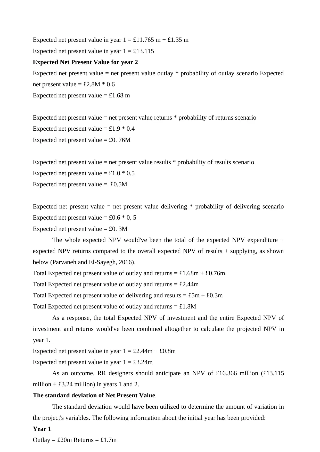
Expected net present value in year 1 = £11.765 m + £1.35 m
Expected net present value in year 1 = £13.115
Expected Net Present Value for year 2
Expected net present value = net present value outlay * probability of outlay scenario Expected
net present value = £2.8M * 0.6
Expected net present value = £1.68 m
Expected net present value = net present value returns * probability of returns scenario
Expected net present value = £1.9 * 0.4
Expected net present value = £0. 76M
Expected net present value = net present value results * probability of results scenario
Expected net present value = £1.0 * 0.5
Expected net present value = £0.5M
Expected net present value = net present value delivering * probability of delivering scenario
Expected net present value = £0.6 * 0. 5
Expected net present value = £0. 3M
The whole expected NPV would've been the total of the expected NPV expenditure +
expected NPV returns compared to the overall expected NPV of results + supplying, as shown
below (Parvaneh and El-Sayegh, 2016).
Total Expected net present value of outlay and returns = £1.68m + £0.76m
Total Expected net present value of outlay and returns = £2.44m
Total Expected net present value of delivering and results = £5m + £0.3m
Total Expected net present value of outlay and returns = £1.8M
As a response, the total Expected NPV of investment and the entire Expected NPV of
investment and returns would've been combined altogether to calculate the projected NPV in
year 1.
Expected net present value in year 1 = £2.44m + £0.8m
Expected net present value in year 1 = £3.24m
As an outcome, RR designers should anticipate an NPV of £16.366 million (£13.115
million + £3.24 million) in years 1 and 2.
The standard deviation of Net Present Value
The standard deviation would have been utilized to determine the amount of variation in
the project's variables. The following information about the initial year has been provided:
Year 1
Outlay = £20m Returns = £1.7m
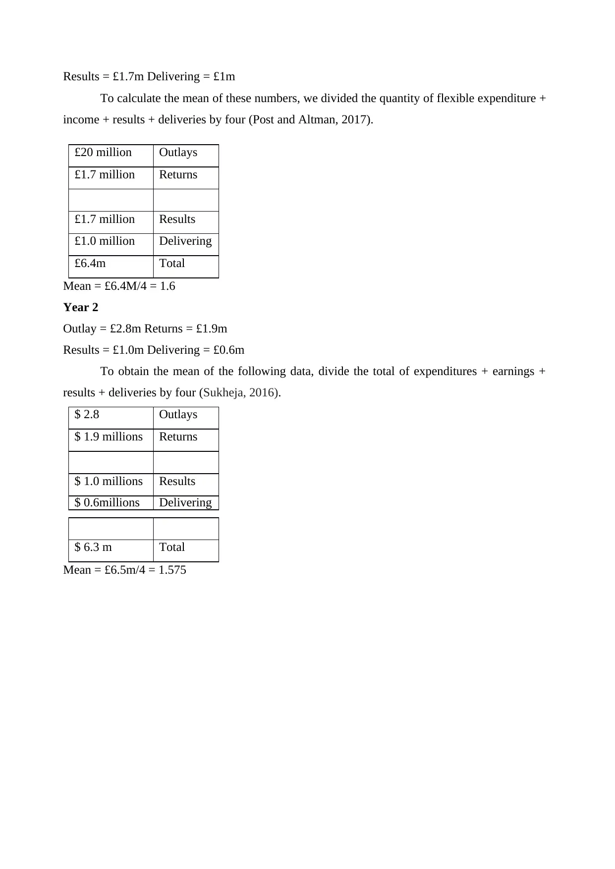
Results = £1.7m Delivering = £1m
To calculate the mean of these numbers, we divided the quantity of flexible expenditure +
income + results + deliveries by four (Post and Altman, 2017).
£20 million Outlays
£1.7 million Returns
£1.7 million Results
£1.0 million Delivering
£6.4m Total
Mean = £6.4M/4 = 1.6
Year 2
Outlay = £2.8m Returns = £1.9m
Results = £1.0m Delivering = £0.6m
To obtain the mean of the following data, divide the total of expenditures + earnings +
results + deliveries by four (Sukheja, 2016).
$ 2.8 Outlays
$ 1.9 millions Returns
$ 1.0 millions Results
$ 0.6millions Delivering
$ 6.3 m Total
Mean = £6.5m/4 = 1.575
⊘ This is a preview!⊘
Do you want full access?
Subscribe today to unlock all pages.

Trusted by 1+ million students worldwide
√
√
√
√
√
√
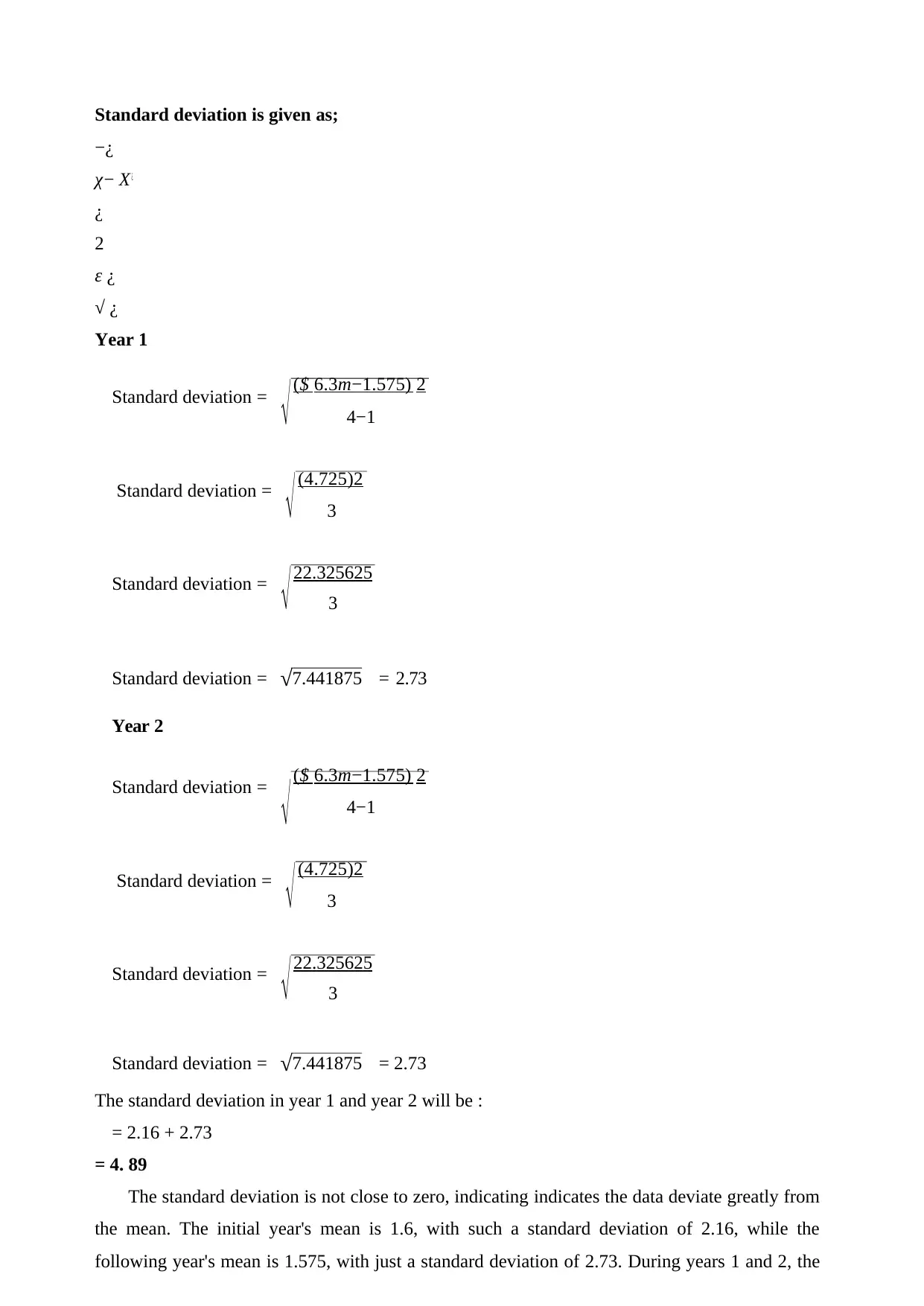
Standard deviation is given as;
−¿
χ− Χ ¿
¿
2
ε ¿
√ ¿
Year 1
Standard deviation = ($ 6.3m−1.575) 2
4−1
Standard deviation = (4.725)2
3
Standard deviation = 22.325625
3
Standard deviation = √7.441875 = 2.73
Year 2
Standard deviation = ($ 6.3m−1.575) 2
4−1
Standard deviation = (4.725)2
3
Standard deviation = 22.325625
3
Standard deviation = √7.441875 = 2.73
The standard deviation in year 1 and year 2 will be :
= 2.16 + 2.73
= 4. 89
The standard deviation is not close to zero, indicating indicates the data deviate greatly from
the mean. The initial year's mean is 1.6, with such a standard deviation of 2.16, while the
following year's mean is 1.575, with just a standard deviation of 2.73. During years 1 and 2, the
√
√
√
√
√
Standard deviation is given as;
−¿
χ− Χ ¿
¿
2
ε ¿
√ ¿
Year 1
Standard deviation = ($ 6.3m−1.575) 2
4−1
Standard deviation = (4.725)2
3
Standard deviation = 22.325625
3
Standard deviation = √7.441875 = 2.73
Year 2
Standard deviation = ($ 6.3m−1.575) 2
4−1
Standard deviation = (4.725)2
3
Standard deviation = 22.325625
3
Standard deviation = √7.441875 = 2.73
The standard deviation in year 1 and year 2 will be :
= 2.16 + 2.73
= 4. 89
The standard deviation is not close to zero, indicating indicates the data deviate greatly from
the mean. The initial year's mean is 1.6, with such a standard deviation of 2.16, while the
following year's mean is 1.575, with just a standard deviation of 2.73. During years 1 and 2, the
Paraphrase This Document
Need a fresh take? Get an instant paraphrase of this document with our AI Paraphraser
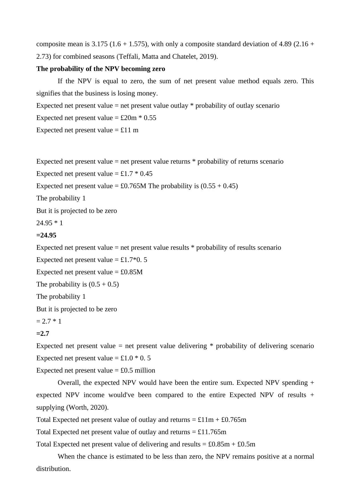
composite mean is 3.175 (1.6 + 1.575), with only a composite standard deviation of 4.89 (2.16 +
2.73) for combined seasons (Teffali, Matta and Chatelet, 2019).
The probability of the NPV becoming zero
If the NPV is equal to zero, the sum of net present value method equals zero. This
signifies that the business is losing money.
Expected net present value = net present value outlay * probability of outlay scenario
Expected net present value = £20m * 0.55
Expected net present value = £11 m
Expected net present value = net present value returns * probability of returns scenario
Expected net present value = £1.7 * 0.45
Expected net present value = £0.765M The probability is (0.55 + 0.45)
The probability 1
But it is projected to be zero
24.95 * 1
=24.95
Expected net present value = net present value results * probability of results scenario
Expected net present value = £1.7*0. 5
Expected net present value = £0.85M
The probability is (0.5 + 0.5)
The probability 1
But it is projected to be zero
= 2.7 * 1
=2.7
Expected net present value = net present value delivering * probability of delivering scenario
Expected net present value = £1.0 * 0. 5
Expected net present value = £0.5 million
Overall, the expected NPV would have been the entire sum. Expected NPV spending +
expected NPV income would've been compared to the entire Expected NPV of results +
supplying (Worth, 2020).
Total Expected net present value of outlay and returns = £11m + £0.765m
Total Expected net present value of outlay and returns = £11.765m
Total Expected net present value of delivering and results = £0.85m + £0.5m
When the chance is estimated to be less than zero, the NPV remains positive at a normal
distribution.
The net present value (NPV) is a way of determining the present value as described in the
following:
The traditional NPV model is essential since it considers the term value of money
through net present value technique. Furthermore, conventional NPV covers both cash flow and
end cash reserves for all periods. As a consequence, NPV investigates the project's future profit.
Furthermore, NPV is a fast way to determine whether an endeavour will be profitable. NPV, on
the other hand, is dependent on the trustworthiness of data in planning and executing informed
evaluations and conclusions. A few of the measures, however, are merely educated assumptions.
Another limitation of NPV is that it cannot be utilized to assess businesses of varying sizes.
Earnings generally seemed to be higher in larger companies. In contrast, NPV indicates that
similar ventures will consistently provide similar outcomes. The typical NPV method for planned
investment calculates NPV by deducting the present value of initial investments from the
expected present value of eventual retained earnings. The WACC is commonly used to
determine reduced prices that are usually risk-adjusted. The WACC is calculated using methods
such as CAPM. This method of calculating NPV assumes that the improvement would
commence as early as possible and continue until it has been done. RR Ltd will come to a
conclusion immediately here, and that decision would've been permanent and irrevocable. The
traditional NPV method restricts management agility. Management may adapt to changing
economic position, such as devaluation, by expanding activities if the firm's overall look is
acceptable, or by curtailing activities if the firm's overall image is unpleasant. Moreover,
traditional NPV overlooks geographical elements of ventures, such as the option to increase into
new territories or introduce new ideas. As a consequence, normal NPV lacks to represent the
nature of risk over a given timeframe (Zimon and Zimon, 2019).
On the other extreme, the viable different solutions method to construction expenditure
takes practical factors of projects into account, such as management flexibility. Unlike traditional
NPV, which believes that investors are inactive, the choice costing system implies that
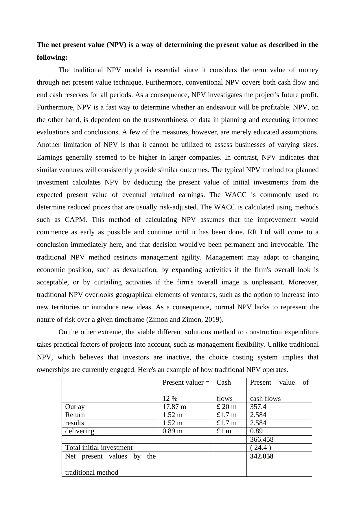
ownerships are currently engaged. Here's an example of how traditional NPV operates.
Present valuer =
12 %
Cash
flows
Present value of
cash flows
Outlay 17.87 m £ 20 m 357.4
Return 1.52 m £1.7 m 2.584
results 1.52 m £1.7 m 2.584
delivering 0.89 m £1 m 0.89
366.458
Total initial investment ( 24.4 )
Net present values by the
traditional method
342.058
⊘ This is a preview!⊘
Do you want full access?
Subscribe today to unlock all pages.

Trusted by 1+ million students worldwide
1 out of 16
Your All-in-One AI-Powered Toolkit for Academic Success.
+13062052269
info@desklib.com
Available 24*7 on WhatsApp / Email
![[object Object]](/_next/static/media/star-bottom.7253800d.svg)
Unlock your academic potential
Copyright © 2020–2026 A2Z Services. All Rights Reserved. Developed and managed by ZUCOL.
