Understanding Hypothesis Tests and Confidence Intervals

This assignment delves into the fundamental concepts of hypothesis testing and confidence intervals. It covers various aspects of statistical inference, including defining hypotheses, determining p-values, calculating confidence intervals, exploring different sampling techniques, and analyzing measures of dispersion such as the coefficient of variation (CV) and range. The assignment aims to enhance your understanding of how to use these statistical tools to draw meaningful conclusions from data.

STUDENT ID
COURSE

INTRODUCTION
We use the dataset of 60 observations given to us for 3 districts to answer a range of questions on
prices across places and other features like ocean view, and type of dwelling-unit or house. The 3
districts covered are Sydney, Wollongong and Newcastle. 2 other categorical variables are provided
for each data point- the type of dwelling can be unit or a house. We are also told about the
absence or presence of ocean view with the dwelling. The focus of the report is on PRICES of
dwellings and how these vary across regions, dwelling type and presence of an ocean view.
We use Microsoft Excel to answer a range of queries pertaining to this data. We use concepts like
measures of central tendency, dispersion, correlation, confidence intervals, and hypothesis testing.
We use t distribution to deal with the hypothesis testing. Visual charts are included - pie chart, bar
chart, and histogram to aid in our analysis.
ANALYSIS:
This section is divided into sub sections, where each subsection deals with a separate query. We
note that we have 4 variables in all, out of which only 1 variable is quantitative. This is prices of
dwellings. All other variables are categorical in nature.
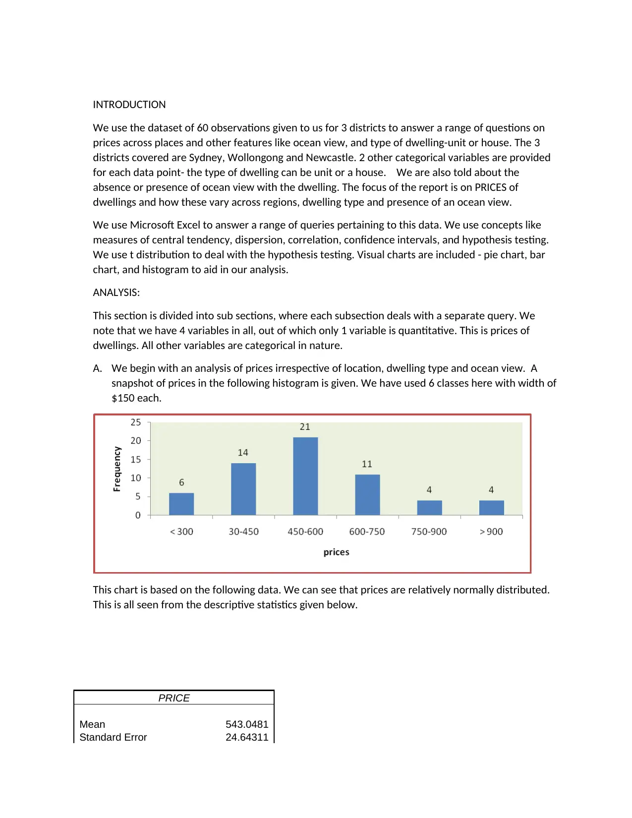
A. We begin with an analysis of prices irrespective of location, dwelling type and ocean view. A
snapshot of prices in the following histogram is given. We have used 6 classes here with width of
$150 each.
This chart is based on the following data. We can see that prices are relatively normally distributed.
This is all seen from the descriptive statistics given below.
PRICE
Mean 543.0481
Standard Error 24.64311

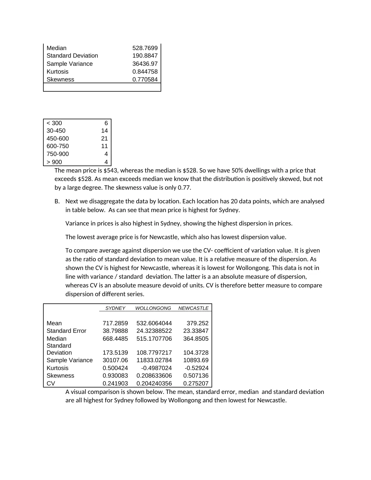
Median 528.7699
Standard Deviation 190.8847
Sample Variance 36436.97
Kurtosis 0.844758
Skewness 0.770584
< 300 6
30-450 14
450-600 21
600-750 11
750-900 4
> 900 4
The mean price is $543, whereas the median is $528. So we have 50% dwellings with a price that
exceeds $528. As mean exceeds median we know that the distribution is positively skewed, but not
by a large degree. The skewness value is only 0.77.
B. Next we disaggregate the data by location. Each location has 20 data points, which are analysed
in table below. As can see that mean price is highest for Sydney.
Variance in prices is also highest in Sydney, showing the highest dispersion in prices.
The lowest average price is for Newcastle, which also has lowest dispersion value.
To compare average against dispersion we use the CV- coefficient of variation value. It is given
as the ratio of standard deviation to mean value. It is a relative measure of the dispersion. As
shown the CV is highest for Newcastle, whereas it is lowest for Wollongong. This data is not in
line with variance / standard deviation. The latter is a an absolute measure of dispersion,
whereas CV is an absolute measure devoid of units. CV is therefore better measure to compare
dispersion of different series.
SYDNEY WOLLONGONG NEWCASTLE
Mean 717.2859 532.6064044 379.252
Standard Error 38.79888 24.32388522 23.33847
Median 668.4485 515.1707706 364.8505
Standard
Deviation 173.5139 108.7797217 104.3728
Sample Variance 30107.06 11833.02784 10893.69
Kurtosis 0.500424 -0.4987024 -0.52924
Skewness 0.930083 0.208633606 0.507136
CV 0.241903 0.204240356 0.275207
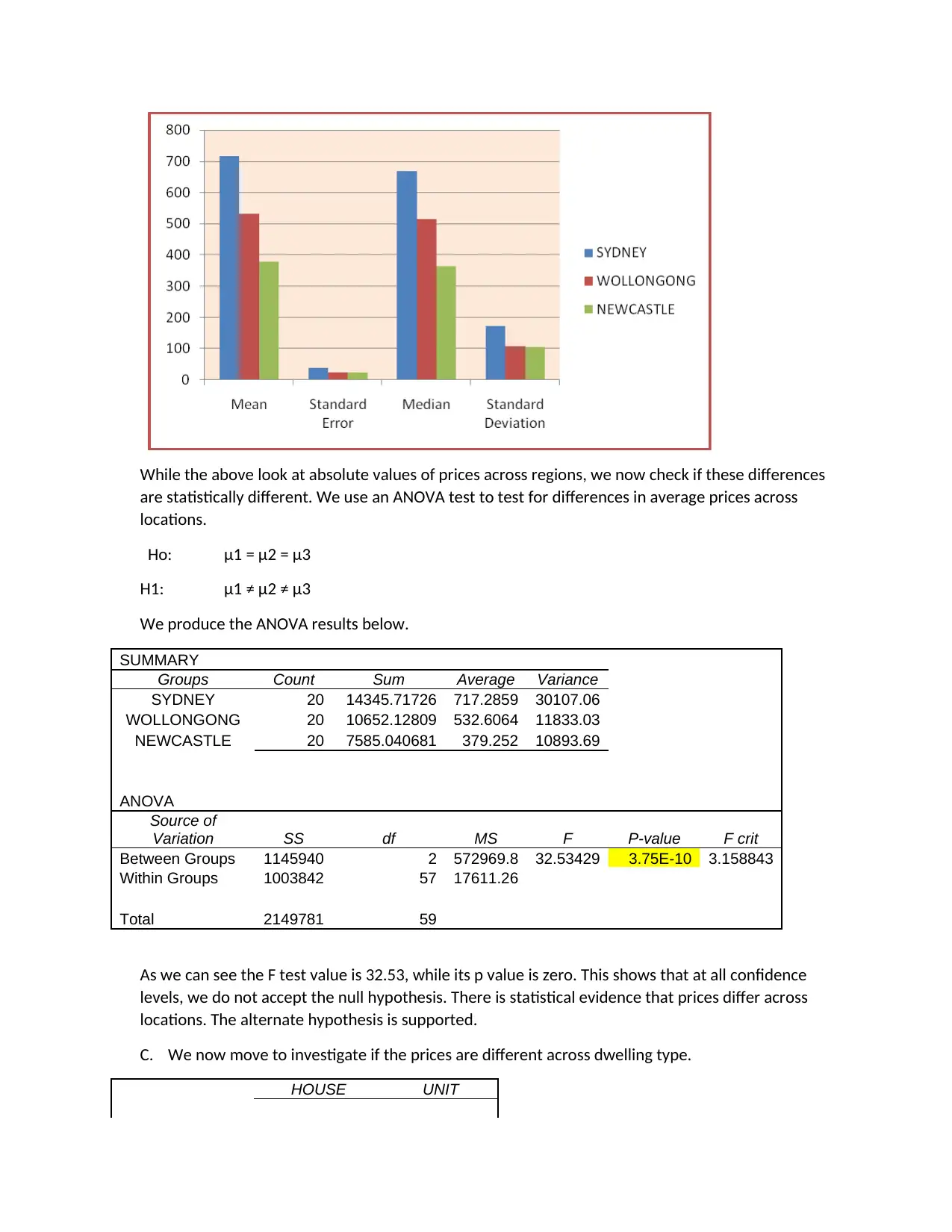
A visual comparison is shown below. The mean, standard error, median and standard deviation
are all highest for Sydney followed by Wollongong and then lowest for Newcastle.

While the above look at absolute values of prices across regions, we now check if these differences
are statistically different. We use an ANOVA test to test for differences in average prices across
locations.
Ho: μ1 = μ2 = μ3
H1: μ1 ≠ μ2 ≠ μ3
We produce the ANOVA results below.
SUMMARY
Groups Count Sum Average Variance
SYDNEY 20 14345.71726 717.2859 30107.06
WOLLONGONG 20 10652.12809 532.6064 11833.03
NEWCASTLE 20 7585.040681 379.252 10893.69
ANOVA
Source of
Variation SS df MS F P-value F crit
Between Groups 1145940 2 572969.8 32.53429 3.75E-10 3.158843
Within Groups 1003842 57 17611.26
Total 2149781 59
As we can see the F test value is 32.53, while its p value is zero. This shows that at all confidence
levels, we do not accept the null hypothesis. There is statistical evidence that prices differ across
locations. The alternate hypothesis is supported.
C. We now move to investigate if the prices are different across dwelling type.
HOUSE UNIT

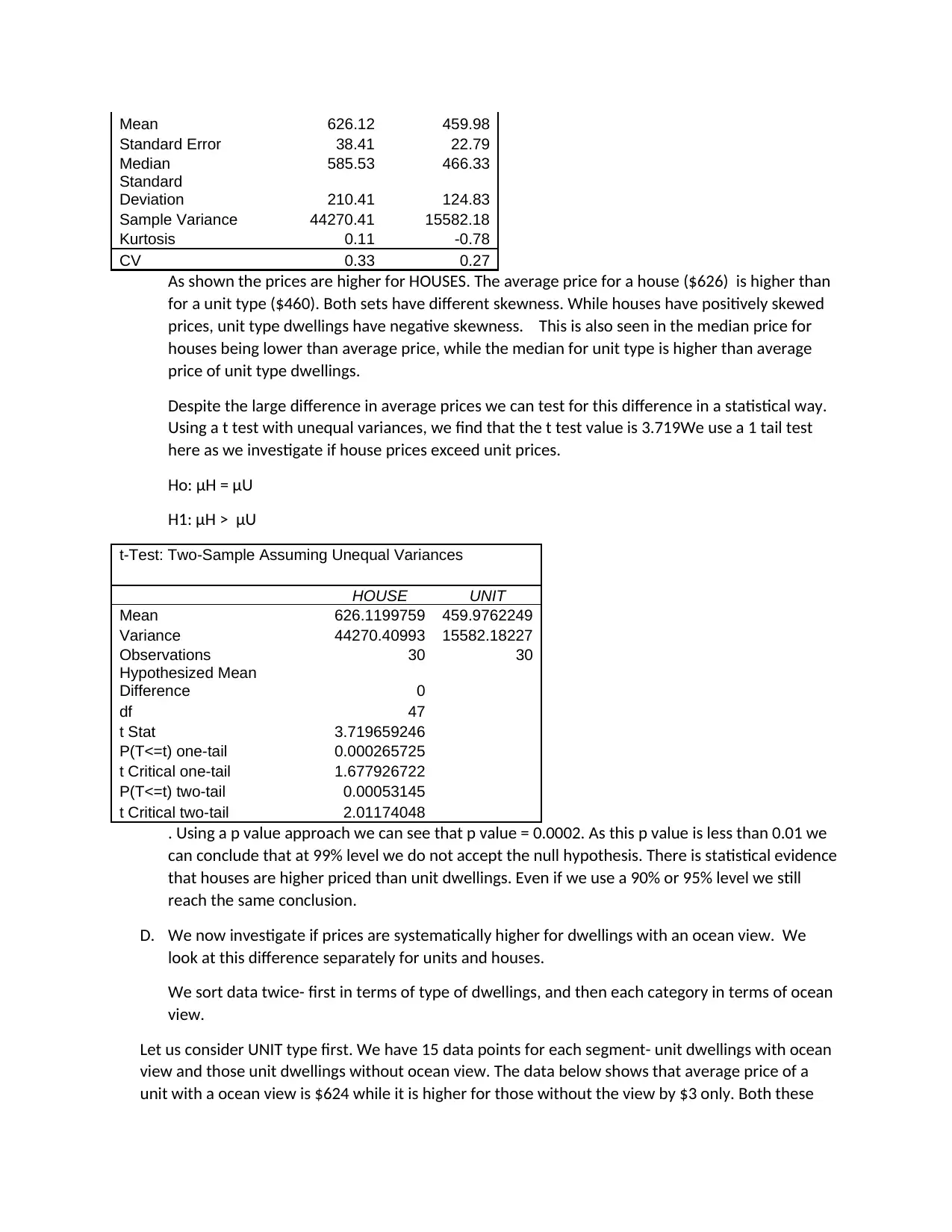
Mean 626.12 459.98
Standard Error 38.41 22.79
Median 585.53 466.33
Standard
Deviation 210.41 124.83
Sample Variance 44270.41 15582.18
Kurtosis 0.11 -0.78
CV 0.33 0.27
As shown the prices are higher for HOUSES. The average price for a house ($626) is higher than
for a unit type ($460). Both sets have different skewness. While houses have positively skewed
prices, unit type dwellings have negative skewness. This is also seen in the median price for
houses being lower than average price, while the median for unit type is higher than average
price of unit type dwellings.
Despite the large difference in average prices we can test for this difference in a statistical way.
Using a t test with unequal variances, we find that the t test value is 3.719We use a 1 tail test
here as we investigate if house prices exceed unit prices.
Ho: μH = μU
H1: μH > μU
t-Test: Two-Sample Assuming Unequal Variances
HOUSE UNIT
Mean 626.1199759 459.9762249
Variance 44270.40993 15582.18227
Observations 30 30
Hypothesized Mean
Difference 0
df 47
t Stat 3.719659246
P(T<=t) one-tail 0.000265725
t Critical one-tail 1.677926722
P(T<=t) two-tail 0.00053145
t Critical two-tail 2.01174048
. Using a p value approach we can see that p value = 0.0002. As this p value is less than 0.01 we
can conclude that at 99% level we do not accept the null hypothesis. There is statistical evidence
that houses are higher priced than unit dwellings. Even if we use a 90% or 95% level we still
reach the same conclusion.
D. We now investigate if prices are systematically higher for dwellings with an ocean view. We
look at this difference separately for units and houses.
We sort data twice- first in terms of type of dwellings, and then each category in terms of ocean
view.
Let us consider UNIT type first. We have 15 data points for each segment- unit dwellings with ocean
view and those unit dwellings without ocean view. The data below shows that average price of a
unit with a ocean view is $624 while it is higher for those without the view by $3 only. Both these

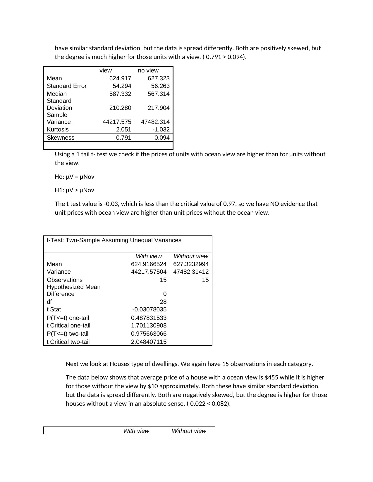
have similar standard deviation, but the data is spread differently. Both are positively skewed, but
the degree is much higher for those units with a view. ( 0.791 > 0.094).
view no view
Mean 624.917 627.323
Standard Error 54.294 56.263
Median 587.332 567.314
Standard
Deviation 210.280 217.904
Sample
Variance 44217.575 47482.314
Kurtosis 2.051 -1.032
Skewness 0.791 0.094
Using a 1 tail t- test we check if the prices of units with ocean view are higher than for units without
the view.
Ho: μV = μNov
H1: μV > μNov
The t test value is -0.03, which is less than the critical value of 0.97. so we have NO evidence that
unit prices with ocean view are higher than unit prices without the ocean view.
t-Test: Two-Sample Assuming Unequal Variances
With view Without view
Mean 624.9166524 627.3232994
Variance 44217.57504 47482.31412
Observations 15 15
Hypothesized Mean
Difference 0
df 28
t Stat -0.03078035
P(T<=t) one-tail 0.487831533
t Critical one-tail 1.701130908
P(T<=t) two-tail 0.975663066
t Critical two-tail 2.048407115
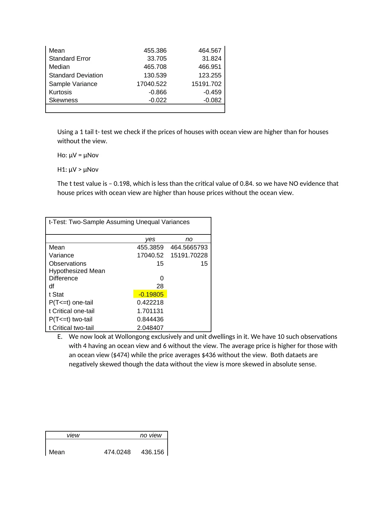
Next we look at Houses type of dwellings. We again have 15 observations in each category.
The data below shows that average price of a house with a ocean view is $455 while it is higher
for those without the view by $10 approximately. Both these have similar standard deviation,
but the data is spread differently. Both are negatively skewed, but the degree is higher for those
houses without a view in an absolute sense. ( 0.022 < 0.082).
With view Without view

Mean 455.386 464.567
Standard Error 33.705 31.824
Median 465.708 466.951
Standard Deviation 130.539 123.255
Sample Variance 17040.522 15191.702
Kurtosis -0.866 -0.459
Skewness -0.022 -0.082
Using a 1 tail t- test we check if the prices of houses with ocean view are higher than for houses
without the view.
Ho: μV = μNov
H1: μV > μNov
The t test value is – 0.198, which is less than the critical value of 0.84. so we have NO evidence that
house prices with ocean view are higher than house prices without the ocean view.
t-Test: Two-Sample Assuming Unequal Variances
yes no
Mean 455.3859 464.5665793
Variance 17040.52 15191.70228
Observations 15 15
Hypothesized Mean
Difference 0
df 28
t Stat -0.19805
P(T<=t) one-tail 0.422218
t Critical one-tail 1.701131
P(T<=t) two-tail 0.844436
t Critical two-tail 2.048407
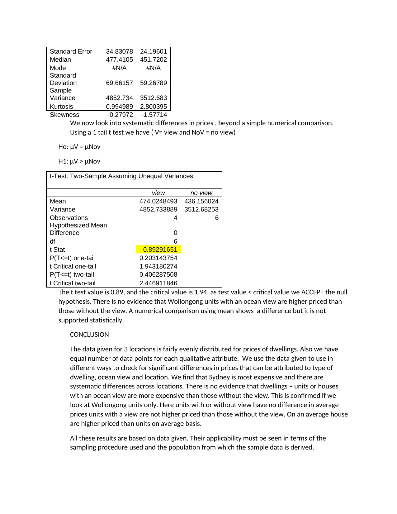
E. We now look at Wollongong exclusively and unit dwellings in it. We have 10 such observations
with 4 having an ocean view and 6 without the view. The average price is higher for those with
an ocean view ($474) while the price averages $436 without the view. Both dataets are
negatively skewed though the data without the view is more skewed in absolute sense.
view no view
Mean 474.0248 436.156

Standard Error 34.83078 24.19601
Median 477.4105 451.7202
Mode #N/A #N/A
Standard
Deviation 69.66157 59.26789
Sample
Variance 4852.734 3512.683
Kurtosis 0.994989 2.800395
Skewness -0.27972 -1.57714
We now look into systematic differences in prices , beyond a simple numerical comparison.
Using a 1 tail t test we have ( V= view and NoV = no view)
Ho: μV = μNov
H1: μV > μNov
t-Test: Two-Sample Assuming Unequal Variances
view no view
Mean 474.0248493 436.156024
Variance 4852.733889 3512.68253
Observations 4 6
Hypothesized Mean
Difference 0
df 6
t Stat 0.89291651
P(T<=t) one-tail 0.203143754
t Critical one-tail 1.943180274
P(T<=t) two-tail 0.406287508
t Critical two-tail 2.446911846
The t test value is 0.89, and the critical value is 1.94. as test value < critical value we ACCEPT the null
hypothesis. There is no evidence that Wollongong units with an ocean view are higher priced than
those without the view. A numerical comparison using mean shows a difference but it is not
supported statistically.
CONCLUSION
The data given for 3 locations is fairly evenly distributed for prices of dwellings. Also we have
equal number of data points for each qualitative attribute. We use the data given to use in
different ways to check for significant differences in prices that can be attributed to type of
dwelling, ocean view and location. We find that Sydney is most expensive and there are
systematic differences across locations. There is no evidence that dwellings – units or houses
with an ocean view are more expensive than those without the view. This is confirmed if we
look at Wollongong units only. Here units with or without view have no difference in average
prices units with a view are not higher priced than those without the view. On an average house
are higher priced than units on average basis.
All these results are based on data given. Their applicability must be seen in terms of the
sampling procedure used and the population from which the sample data is derived.

Anon., n.d. choosing the number of bins. [Online] Available
athttp://statweb.stanford.edu/~susan/courses/s60/split/node43.html [Accessed 9 Oct 2017].
Anon., n.d. How to choose no of bins. [Online] [Accessed 11 Oct 2017].
Anon., n.d. Hypothesis Testing. [Online] Available at:
https://onlinecourses.science.psu.edu/statprogram/node/138 [Accessed 14 Oct 2017].
Anon., n.d. Hypothess testing. [Online] Available athttp://www.statisticshowto.com/probability-and-
statistics/hypothesis-testing/ [Accessed 21 Oct 2017].
Anon., n.d. Mean, median, mode. [Online] Available at:
http://www.bbc.co.uk/schools/gcsebitesize/maths/statistics/measuresofaveragerev6.shtml
[Accessed 12 Oct 2017].
Cfcc.edu, n.d. Tests of hypothesis. [Online] Available at: http://cfcc.edu/faculty/cmoore/0801-
HypothesisTests.pdf [Accessed 15 Oct 2017].
Cyclismo.org, n.d. calculating confidence intervals. [Online] Available
athttp://www.cyclismo.org/tutorial/R/confidence.html [Accessed 15 Oct 2017].
Insee.fr, 2016. Coefficeient of Varaiation/CV. [Online] Available
athttps://www.insee.fr/en/metadonnees/definition/c1366 [Accessed 11 Oct 2017].
Kean.edu, n.d. Confidence Inteval for Mean. [Online] Available
athttp://www.kean.edu/~fosborne/bstat/06amean.html [Accessed 16 Oct 2017].
Learn,bu.edu, n.d. The 5 steps in Hypothesis testing. [Online] Available
athttps://learn.bu.edu/bbcswebdav/pid-826908-dt-content-rid-2073693_1/courses/
13sprgmetcj702_ol/week04/metcj702_W04S01T05_fivesteps.html [Accessed 14 Oct 2017].
LEarn.bu.edu, n.d. The fice steps for hypothesis testing. [Online] Available at:
https://learn.bu.edu/bbcswebdav/pid-826908-dt-content-rid-2073693_1/courses/
13sprgmetcj702_ol/week04/metcj702_W04S01T05_fivesteps.html [Accessed 13 Oct 2017].
Online courses.science.psu.edu, n.d. Interval estimate of population mean. [Online] Available at:
https://onlinecourses.science.psu.edu/stat505/node/61 [Accessed 17 Oct 2017].
Rgs.org, n.d. Sampling techniques. [Online] Available at:
http://www.rgs.org/OurWork/Schools/Fieldwork+and+local+learning/Fieldwork+techniques/
Sampling+techniques.htm [Accessed 18 Oct 2017].
Simon.cs.vt.edu, n.d. Measuresof dispersion. [Online] Available
athttps://simon.cs.vt.edu/SoSci/converted/Dispersion_I/ [Accessed 17 Oct 2017].
stat.yale.edu, n.d. Sampliing in Statistical Inference. [Online] Available at:
http://www.stat.yale.edu/Courses/1997-98/101/sampinf.htm [Accessed 17 Oct 2017].

Statistics. laerd.com, n.d. Measures of Spread. [Online] Available at:
https://statistics.laerd.com/statistical-guides/measures-of-spread-range-quartiles.php [Accessed 17
Oct 2017].