Data Analysis Report
VerifiedAdded on 2023/01/11
|52
|5445
|70
AI Summary
This data analysis report covers various topics such as acceptance of nuclear power, climate change, and more. It explores the associations between different variables and their significance. The report includes chi-square tests, correlation analysis, and interpretation of the results.
Contribute Materials
Your contribution can guide someone’s learning journey. Share your
documents today.

Data Analysis Report
Secure Best Marks with AI Grader
Need help grading? Try our AI Grader for instant feedback on your assignments.
TABLE OF CONTENTS
QUESTION 1.............................................................................................................................4
a. Association between the age of respondents with acceptance of nuclear power than to
live..........................................................................................................................................4
B. Association between the age of respondents and good things about a nuclear power......4
C. Association between age of respondents and promoting the renewable energy sources. .4
d. Association between qualification and risk of people in Britain about nuclear power......5
QUESTION 2.............................................................................................................................5
QUESTION 3...........................................................................................................................12
a. Association between age of respondents and pattern of weather is changing..................12
b. Association between qualification of respondents and climate change is inevitable.......13
c. Association between gender of respondents and tackle to climate change......................14
d. Relationship between respondents who experience flood damage and whether they felt
climate change......................................................................................................................14
QUESTION 4...........................................................................................................................15
Appendix..................................................................................................................................37
Q1.........................................................................................................................................37
a)...........................................................................................................................................37
b)..........................................................................................................................................37
c)...........................................................................................................................................38
d)..........................................................................................................................................39
Q2.........................................................................................................................................39

Q3.........................................................................................................................................41
a)...........................................................................................................................................41
b)..........................................................................................................................................43
c)...........................................................................................................................................45
d)..........................................................................................................................................46
Q4.........................................................................................................................................47
QUESTION 1
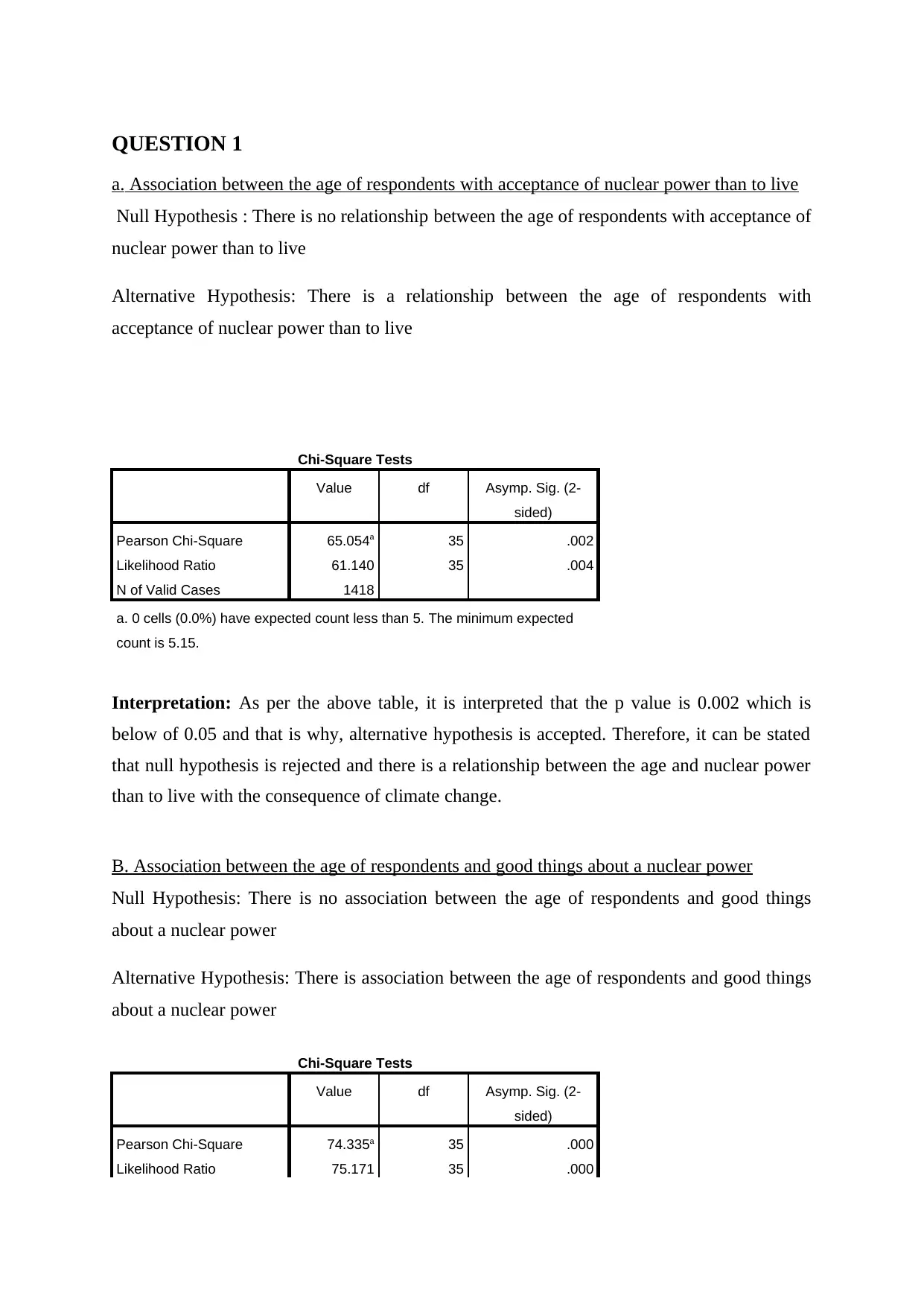
a. Association between the age of respondents with acceptance of nuclear power than to live
Null Hypothesis : There is no relationship between the age of respondents with acceptance of
nuclear power than to live
Alternative Hypothesis: There is a relationship between the age of respondents with
acceptance of nuclear power than to live
Chi-Square Tests
Value df Asymp. Sig. (2-
sided)
Pearson Chi-Square 65.054a 35 .002
Likelihood Ratio 61.140 35 .004
N of Valid Cases 1418
a. 0 cells (0.0%) have expected count less than 5. The minimum expected
count is 5.15.
Interpretation: As per the above table, it is interpreted that the p value is 0.002 which is
below of 0.05 and that is why, alternative hypothesis is accepted. Therefore, it can be stated
that null hypothesis is rejected and there is a relationship between the age and nuclear power
than to live with the consequence of climate change.
B. Association between the age of respondents and good things about a nuclear power
Null Hypothesis: There is no association between the age of respondents and good things
about a nuclear power
Alternative Hypothesis: There is association between the age of respondents and good things
about a nuclear power
Chi-Square Tests
Value df Asymp. Sig. (2-
sided)
Pearson Chi-Square 74.335a 35 .000
Likelihood Ratio 75.171 35 .000
Secure Best Marks with AI Grader
Need help grading? Try our AI Grader for instant feedback on your assignments.
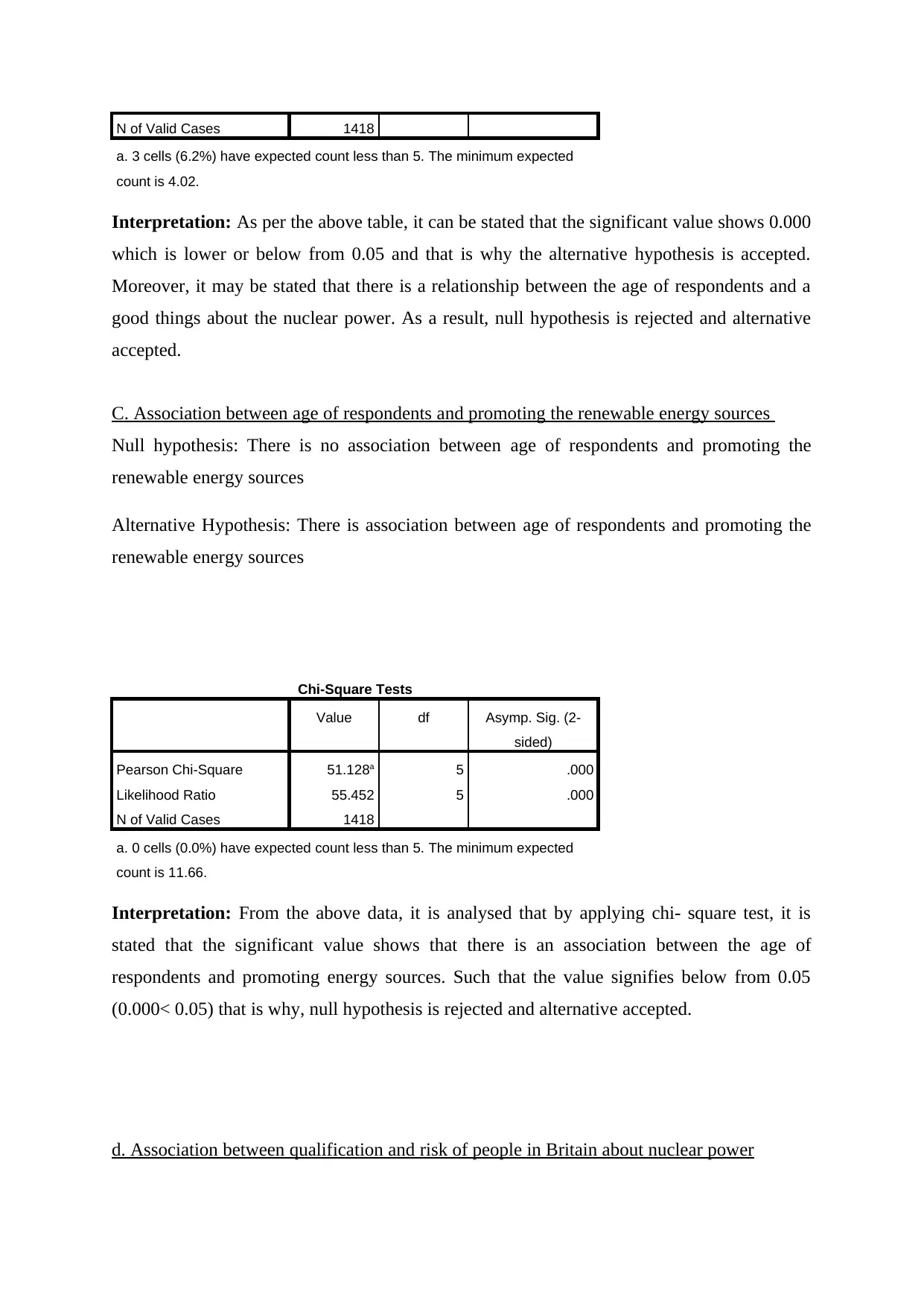
N of Valid Cases 1418
a. 3 cells (6.2%) have expected count less than 5. The minimum expected
count is 4.02.
Interpretation: As per the above table, it can be stated that the significant value shows 0.000
which is lower or below from 0.05 and that is why the alternative hypothesis is accepted.
Moreover, it may be stated that there is a relationship between the age of respondents and a
good things about the nuclear power. As a result, null hypothesis is rejected and alternative
accepted.
C. Association between age of respondents and promoting the renewable energy sources
Null hypothesis: There is no association between age of respondents and promoting the
renewable energy sources
Alternative Hypothesis: There is association between age of respondents and promoting the
renewable energy sources
Chi-Square Tests
Value df Asymp. Sig. (2-
sided)
Pearson Chi-Square 51.128a 5 .000
Likelihood Ratio 55.452 5 .000
N of Valid Cases 1418
a. 0 cells (0.0%) have expected count less than 5. The minimum expected
count is 11.66.
Interpretation: From the above data, it is analysed that by applying chi- square test, it is
stated that the significant value shows that there is an association between the age of
respondents and promoting energy sources. Such that the value signifies below from 0.05
(0.000< 0.05) that is why, null hypothesis is rejected and alternative accepted.
d. Association between qualification and risk of people in Britain about nuclear power
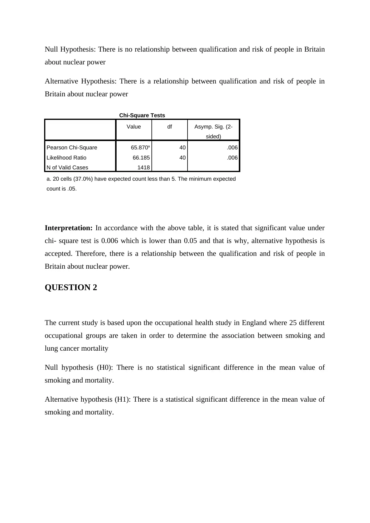
Null Hypothesis: There is no relationship between qualification and risk of people in Britain
about nuclear power
Alternative Hypothesis: There is a relationship between qualification and risk of people in
Britain about nuclear power
Chi-Square Tests
Value df Asymp. Sig. (2-
sided)
Pearson Chi-Square 65.870a 40 .006
Likelihood Ratio 66.185 40 .006
N of Valid Cases 1418
a. 20 cells (37.0%) have expected count less than 5. The minimum expected
count is .05.
Interpretation: In accordance with the above table, it is stated that significant value under
chi- square test is 0.006 which is lower than 0.05 and that is why, alternative hypothesis is
accepted. Therefore, there is a relationship between the qualification and risk of people in
Britain about nuclear power.
QUESTION 2
The current study is based upon the occupational health study in England where 25 different
occupational groups are taken in order to determine the association between smoking and
lung cancer mortality
Null hypothesis (H0): There is no statistical significant difference in the mean value of
smoking and mortality.
Alternative hypothesis (H1): There is a statistical significant difference in the mean value of
smoking and mortality.
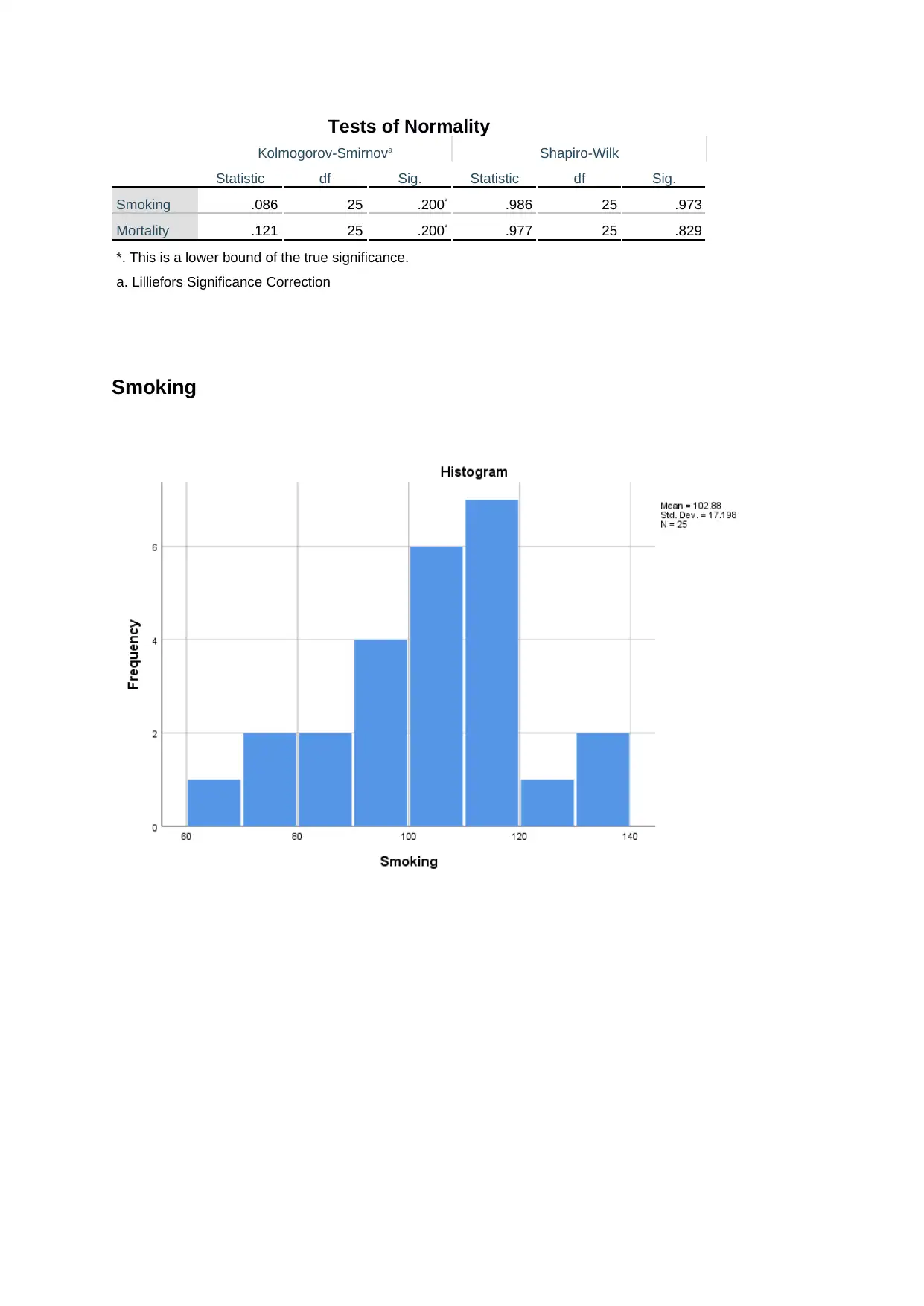
Tests of Normality
Kolmogorov-Smirnova Shapiro-Wilk
Statistic df Sig. Statistic df Sig.
Smoking .086 25 .200* .986 25 .973
Mortality .121 25 .200* .977 25 .829
*. This is a lower bound of the true significance.
a. Lilliefors Significance Correction
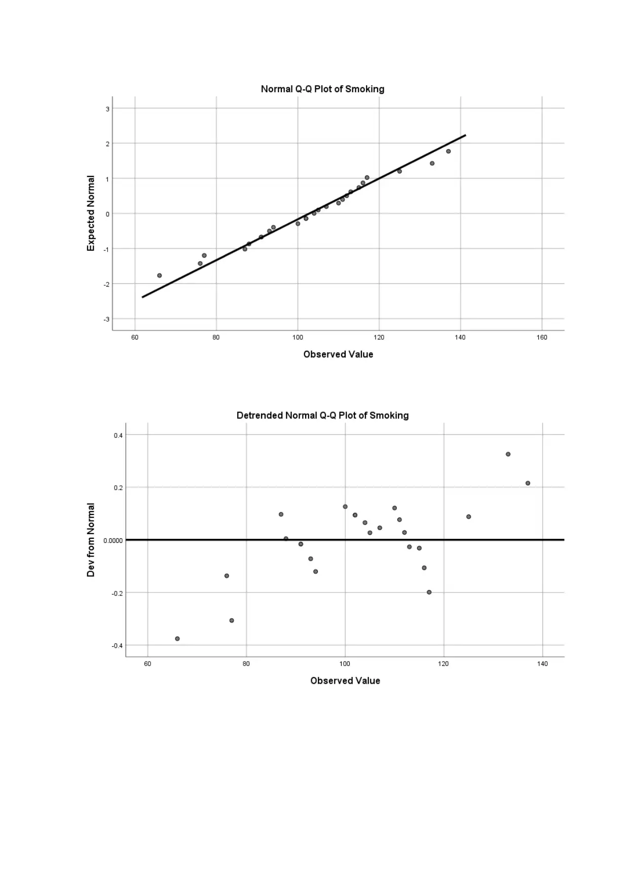
Smoking
Kolmogorov-Smirnova Shapiro-Wilk
Statistic df Sig. Statistic df Sig.
Smoking .086 25 .200* .986 25 .973
Mortality .121 25 .200* .977 25 .829
*. This is a lower bound of the true significance.
a. Lilliefors Significance Correction
Smoking
Paraphrase This Document
Need a fresh take? Get an instant paraphrase of this document with our AI Paraphraser
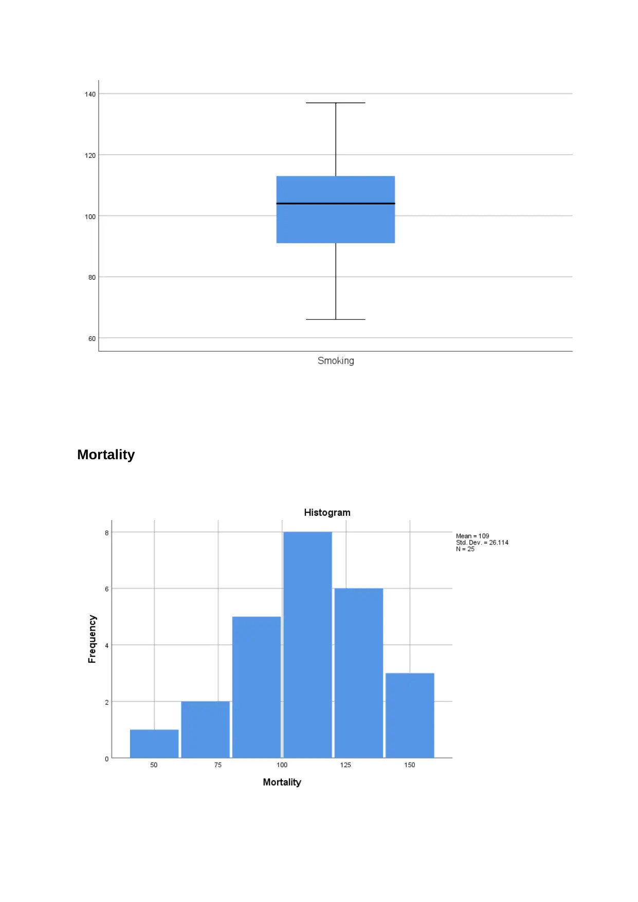
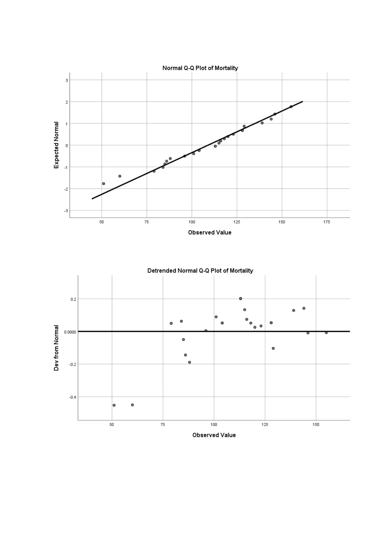
Mortality
Secure Best Marks with AI Grader
Need help grading? Try our AI Grader for instant feedback on your assignments.
Correlations
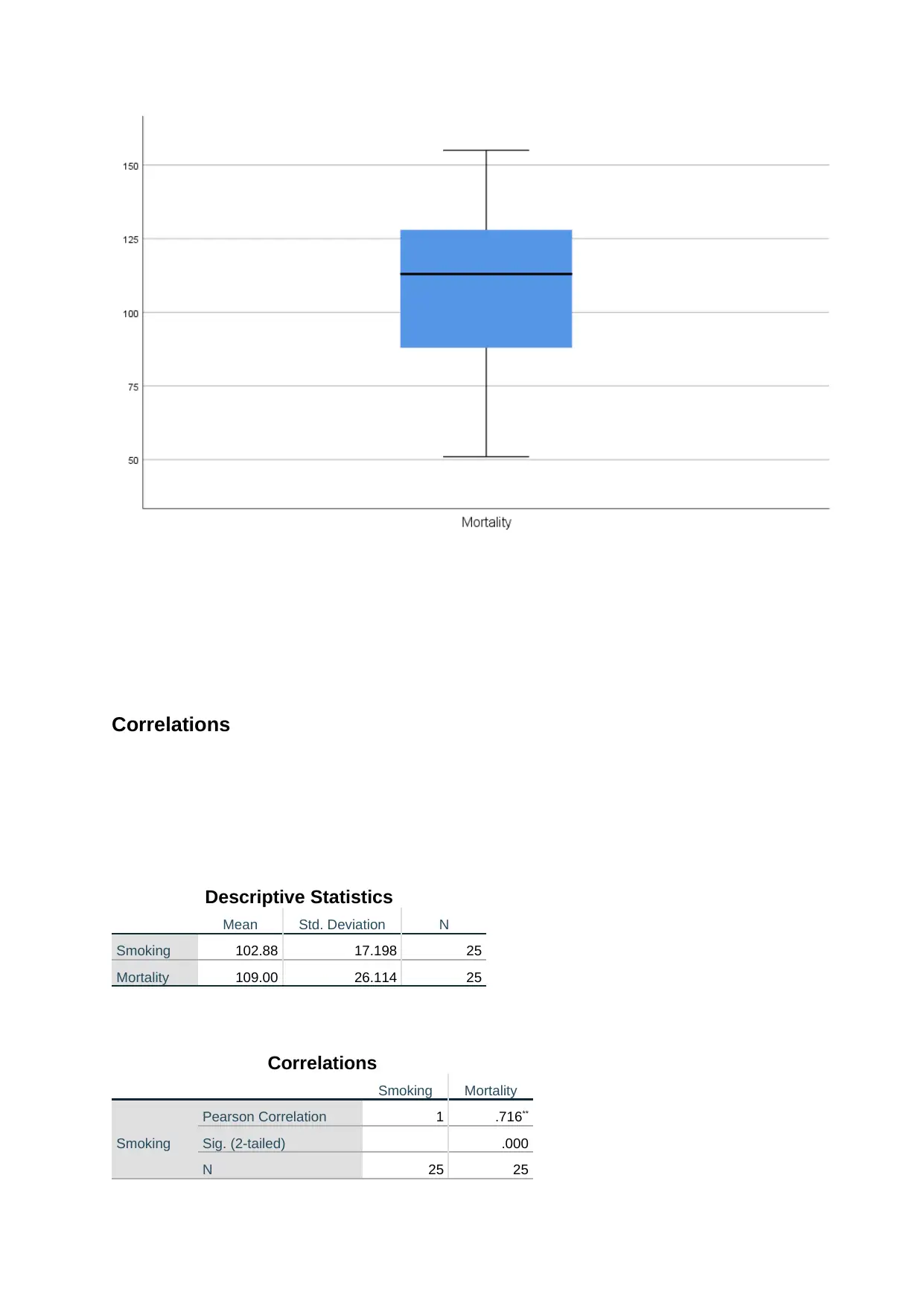
Descriptive Statistics
Mean Std. Deviation N
Smoking 102.88 17.198 25
Mortality 109.00 26.114 25
Correlations
Smoking Mortality
Smoking
Pearson Correlation 1 .716**
Sig. (2-tailed) .000
N 25 25
Descriptive Statistics
Mean Std. Deviation N
Smoking 102.88 17.198 25
Mortality 109.00 26.114 25
Correlations
Smoking Mortality
Smoking
Pearson Correlation 1 .716**
Sig. (2-tailed) .000
N 25 25
Mortality
Pearson Correlation .716** 1
Sig. (2-tailed) .000
N 25 25
**. Correlation is significant at the 0.01 level (2-tailed).
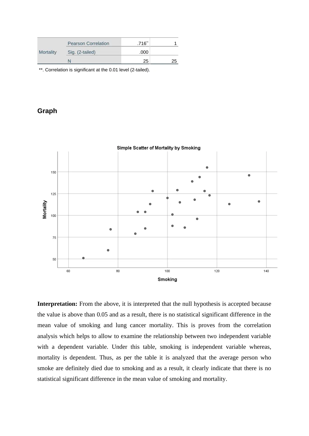
Graph
Interpretation: From the above, it is interpreted that the null hypothesis is accepted because
the value is above than 0.05 and as a result, there is no statistical significant difference in the
mean value of smoking and lung cancer mortality. This is proves from the correlation
analysis which helps to allow to examine the relationship between two independent variable
with a dependent variable. Under this table, smoking is independent variable whereas,
mortality is dependent. Thus, as per the table it is analyzed that the average person who
smoke are definitely died due to smoking and as a result, it clearly indicate that there is no
statistical significant difference in the mean value of smoking and mortality.
Pearson Correlation .716** 1
Sig. (2-tailed) .000
N 25 25
**. Correlation is significant at the 0.01 level (2-tailed).
Graph
Interpretation: From the above, it is interpreted that the null hypothesis is accepted because
the value is above than 0.05 and as a result, there is no statistical significant difference in the
mean value of smoking and lung cancer mortality. This is proves from the correlation
analysis which helps to allow to examine the relationship between two independent variable
with a dependent variable. Under this table, smoking is independent variable whereas,
mortality is dependent. Thus, as per the table it is analyzed that the average person who
smoke are definitely died due to smoking and as a result, it clearly indicate that there is no
statistical significant difference in the mean value of smoking and mortality.
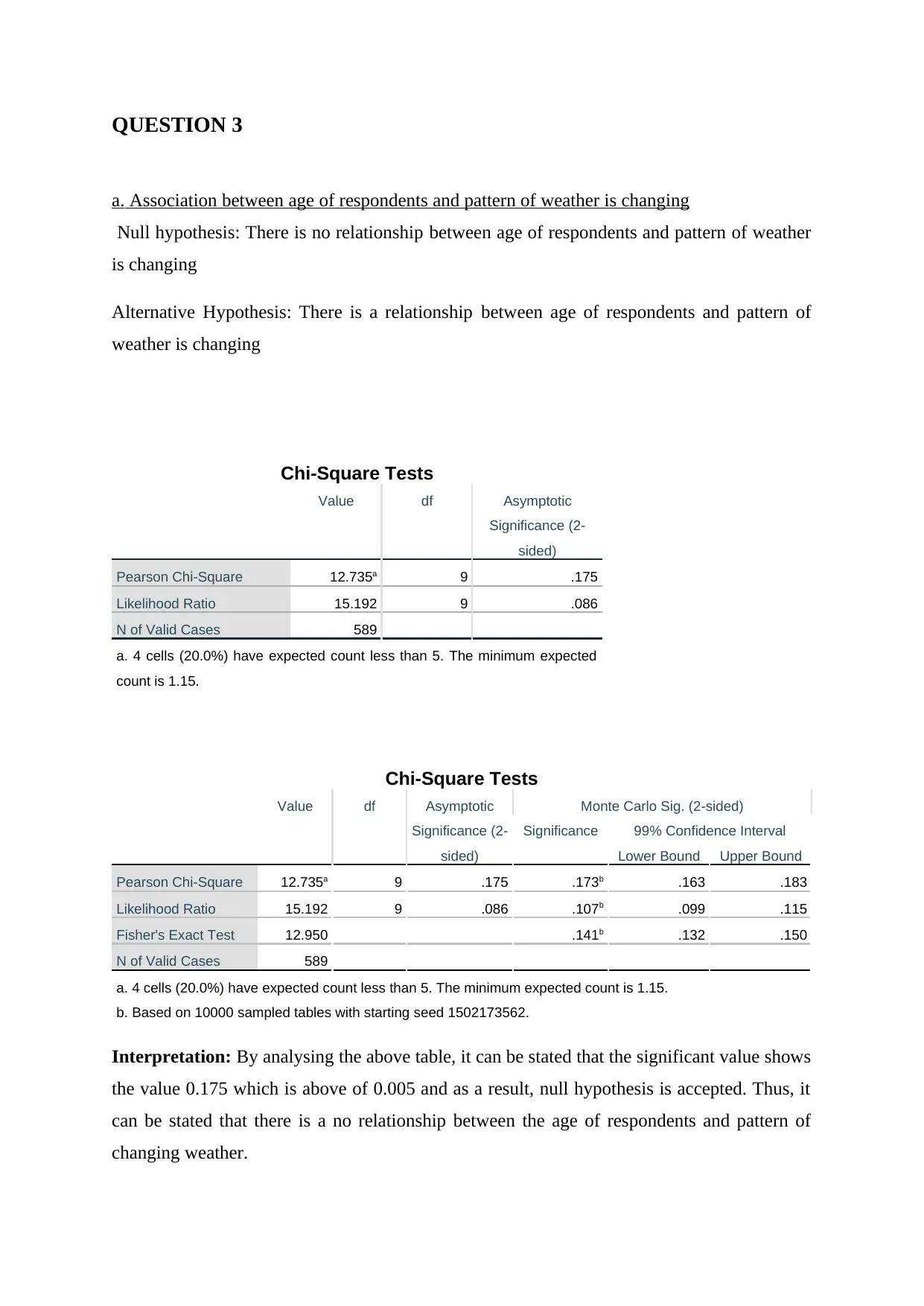
QUESTION 3
a. Association between age of respondents and pattern of weather is changing
Null hypothesis: There is no relationship between age of respondents and pattern of weather
is changing
Alternative Hypothesis: There is a relationship between age of respondents and pattern of
weather is changing
Chi-Square Tests
Value df Asymptotic
Significance (2-
sided)
Pearson Chi-Square 12.735a 9 .175
Likelihood Ratio 15.192 9 .086
N of Valid Cases 589
a. 4 cells (20.0%) have expected count less than 5. The minimum expected
count is 1.15.
Chi-Square Tests
Value df Asymptotic
Significance (2-
sided)
Monte Carlo Sig. (2-sided)
Significance 99% Confidence Interval
Lower Bound Upper Bound
Pearson Chi-Square 12.735a 9 .175 .173b .163 .183
Likelihood Ratio 15.192 9 .086 .107b .099 .115
Fisher's Exact Test 12.950 .141b .132 .150
N of Valid Cases 589
a. 4 cells (20.0%) have expected count less than 5. The minimum expected count is 1.15.
b. Based on 10000 sampled tables with starting seed 1502173562.
Interpretation: By analysing the above table, it can be stated that the significant value shows
the value 0.175 which is above of 0.005 and as a result, null hypothesis is accepted. Thus, it
can be stated that there is a no relationship between the age of respondents and pattern of
changing weather.
Paraphrase This Document
Need a fresh take? Get an instant paraphrase of this document with our AI Paraphraser
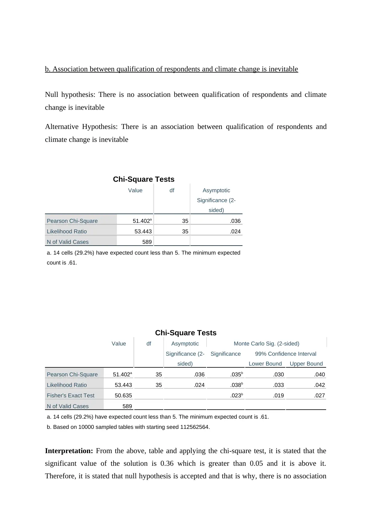
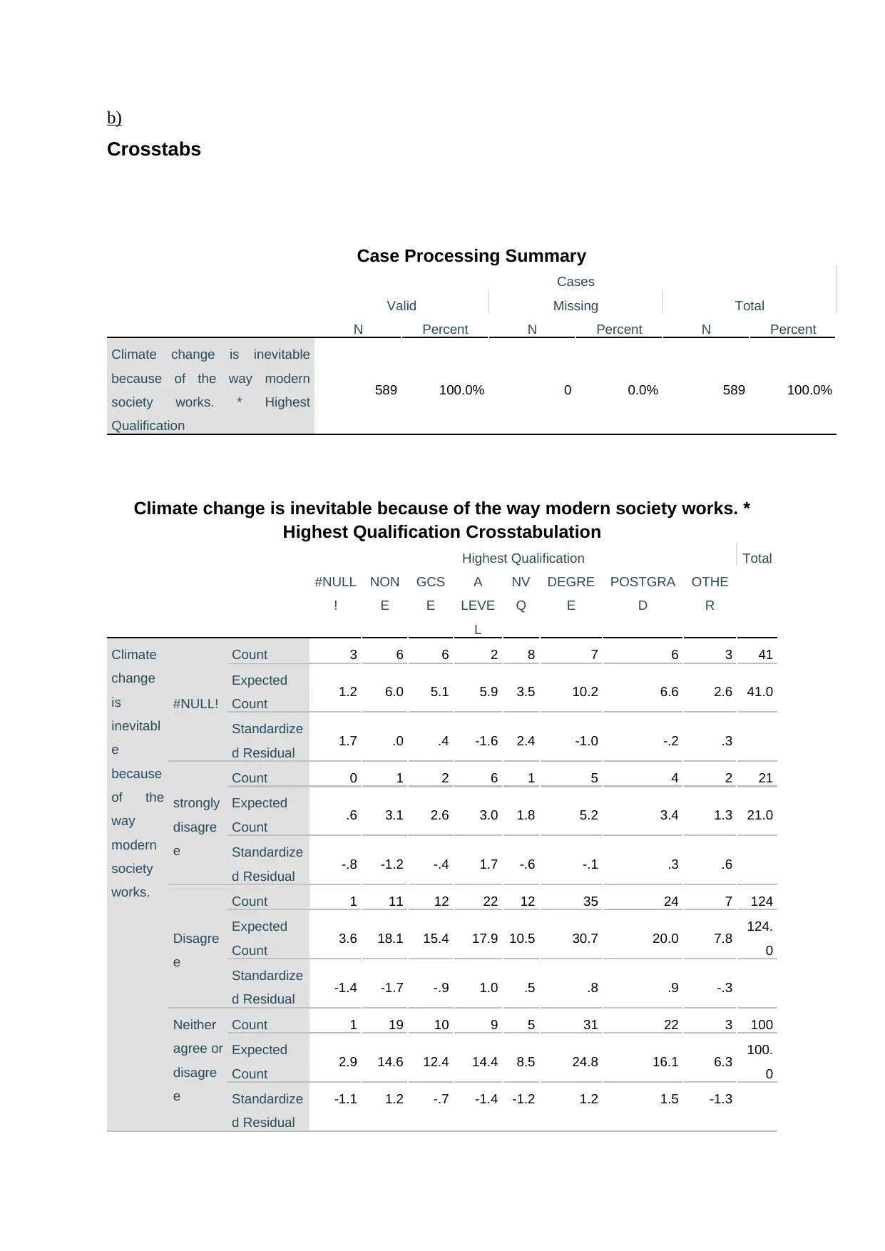
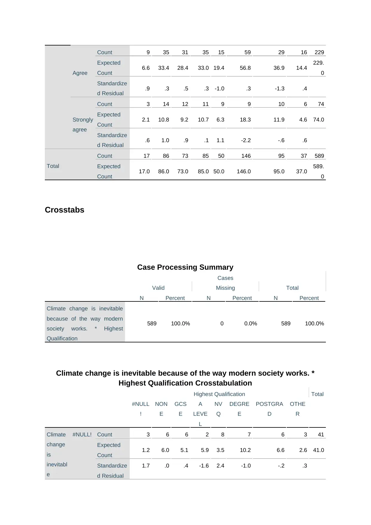
b. Association between qualification of respondents and climate change is inevitable
Null hypothesis: There is no association between qualification of respondents and climate
change is inevitable
Alternative Hypothesis: There is an association between qualification of respondents and
climate change is inevitable
Chi-Square Tests
Value df Asymptotic
Significance (2-
sided)
Pearson Chi-Square 51.402a 35 .036
Likelihood Ratio 53.443 35 .024
N of Valid Cases 589
a. 14 cells (29.2%) have expected count less than 5. The minimum expected
count is .61.
Chi-Square Tests
Value df Asymptotic
Significance (2-
sided)
Monte Carlo Sig. (2-sided)
Significance 99% Confidence Interval
Lower Bound Upper Bound
Pearson Chi-Square 51.402a 35 .036 .035b .030 .040
Likelihood Ratio 53.443 35 .024 .038b .033 .042
Fisher's Exact Test 50.635 .023b .019 .027
N of Valid Cases 589
a. 14 cells (29.2%) have expected count less than 5. The minimum expected count is .61.
b. Based on 10000 sampled tables with starting seed 112562564.
Interpretation: From the above, table and applying the chi-square test, it is stated that the
significant value of the solution is 0.36 which is greater than 0.05 and it is above it.
Therefore, it is stated that null hypothesis is accepted and that is why, there is no association
between the qualification of respondents and climate change, thus alternative hypothesis is
rejected.
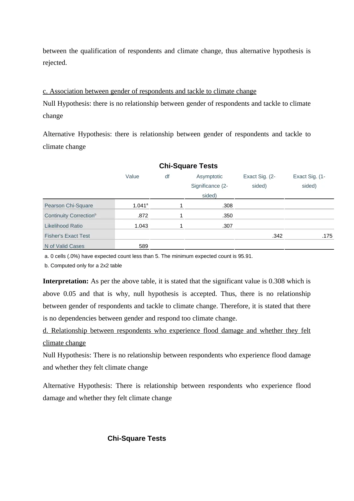
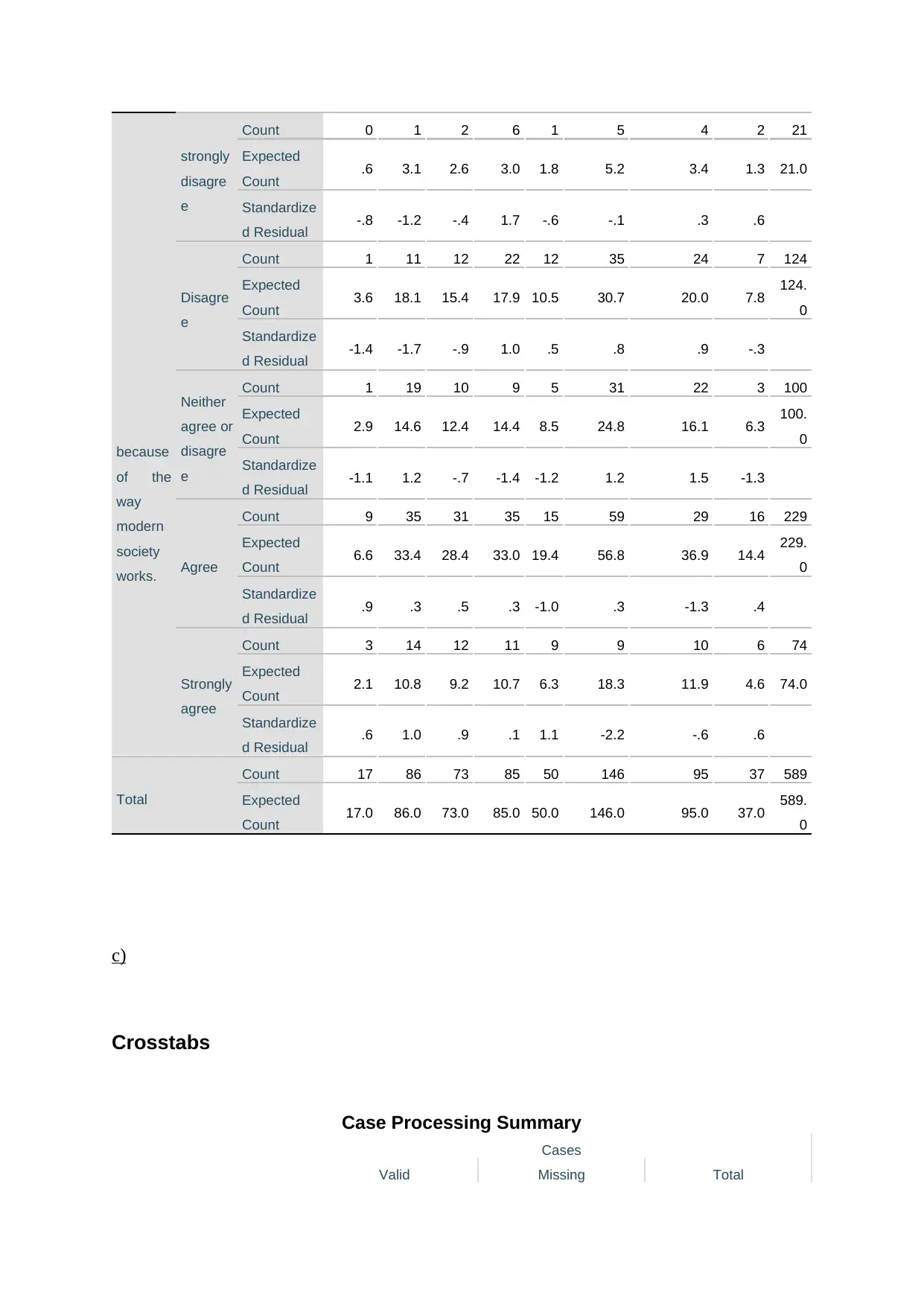
c. Association between gender of respondents and tackle to climate change
Null Hypothesis: there is no relationship between gender of respondents and tackle to climate
change
Alternative Hypothesis: there is relationship between gender of respondents and tackle to
climate change
Chi-Square Tests
Value df Asymptotic
Significance (2-
sided)
Exact Sig. (2-
sided)
Exact Sig. (1-
sided)
Pearson Chi-Square 1.041a 1 .308
Continuity Correctionb .872 1 .350
Likelihood Ratio 1.043 1 .307
Fisher's Exact Test .342 .175
N of Valid Cases 589
a. 0 cells (.0%) have expected count less than 5. The minimum expected count is 95.91.
b. Computed only for a 2x2 table
Interpretation: As per the above table, it is stated that the significant value is 0.308 which is
above 0.05 and that is why, null hypothesis is accepted. Thus, there is no relationship
between gender of respondents and tackle to climate change. Therefore, it is stated that there
is no dependencies between gender and respond too climate change.
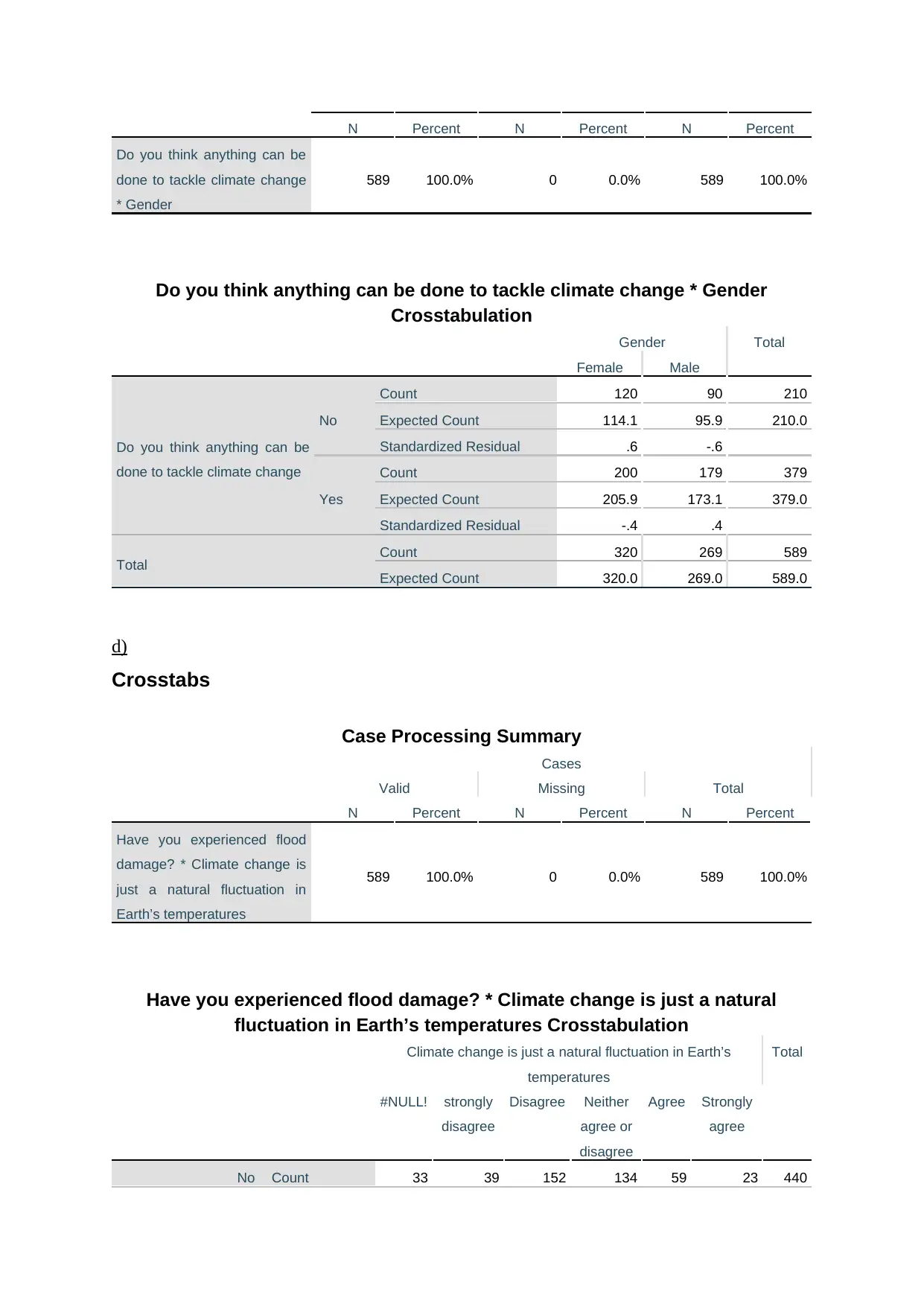
d. Relationship between respondents who experience flood damage and whether they felt
climate change
Null Hypothesis: There is no relationship between respondents who experience flood damage
and whether they felt climate change
Alternative Hypothesis: There is relationship between respondents who experience flood
damage and whether they felt climate change
Chi-Square Tests
rejected.
c. Association between gender of respondents and tackle to climate change
Null Hypothesis: there is no relationship between gender of respondents and tackle to climate
change
Alternative Hypothesis: there is relationship between gender of respondents and tackle to
climate change
Chi-Square Tests
Value df Asymptotic
Significance (2-
sided)
Exact Sig. (2-
sided)
Exact Sig. (1-
sided)
Pearson Chi-Square 1.041a 1 .308
Continuity Correctionb .872 1 .350
Likelihood Ratio 1.043 1 .307
Fisher's Exact Test .342 .175
N of Valid Cases 589
a. 0 cells (.0%) have expected count less than 5. The minimum expected count is 95.91.
b. Computed only for a 2x2 table
Interpretation: As per the above table, it is stated that the significant value is 0.308 which is
above 0.05 and that is why, null hypothesis is accepted. Thus, there is no relationship
between gender of respondents and tackle to climate change. Therefore, it is stated that there
is no dependencies between gender and respond too climate change.
d. Relationship between respondents who experience flood damage and whether they felt
climate change
Null Hypothesis: There is no relationship between respondents who experience flood damage
and whether they felt climate change
Alternative Hypothesis: There is relationship between respondents who experience flood
damage and whether they felt climate change
Chi-Square Tests
Value df Asymptotic
Significance (2-
sided)
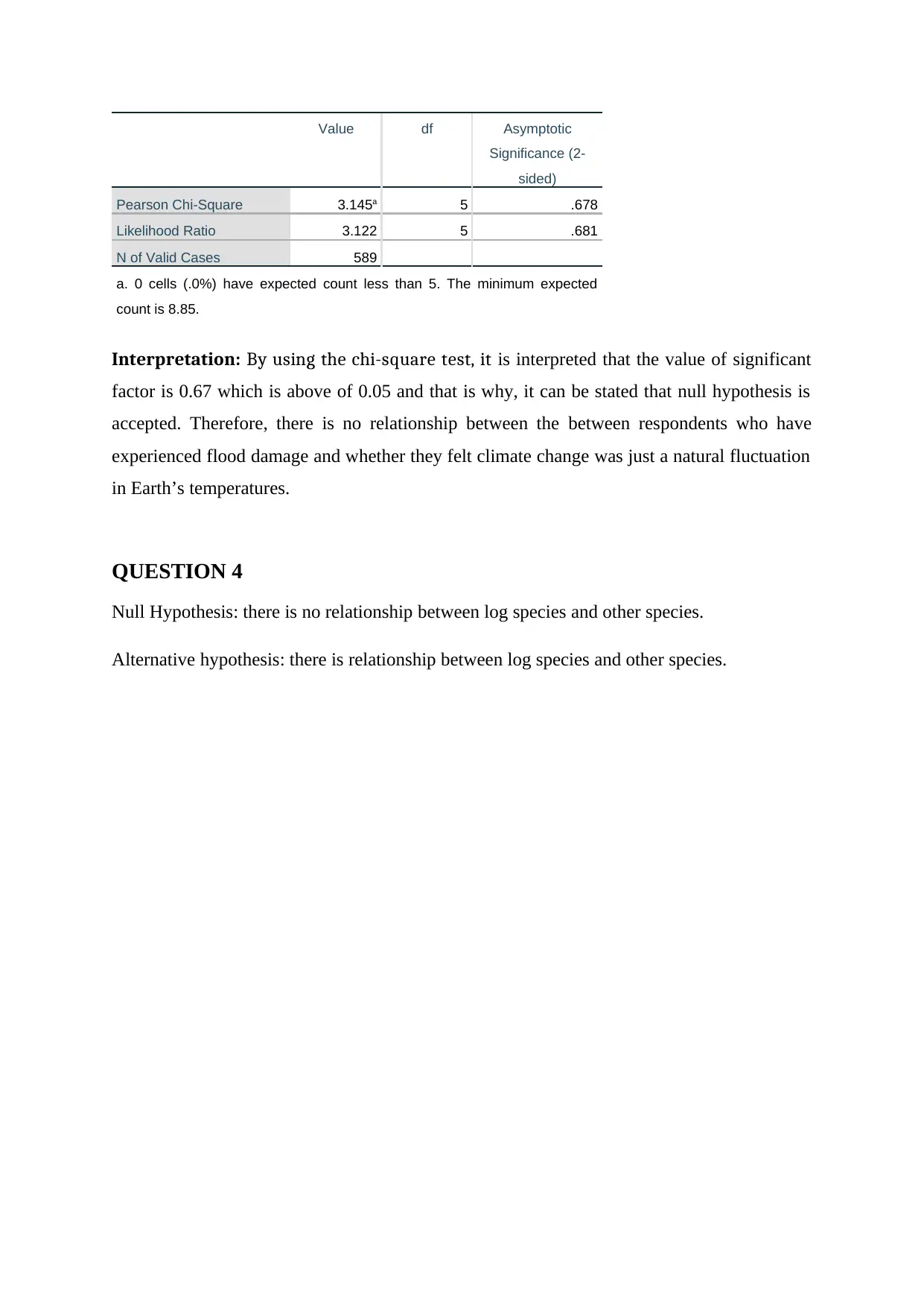
Pearson Chi-Square 3.145a 5 .678
Likelihood Ratio 3.122 5 .681
N of Valid Cases 589
a. 0 cells (.0%) have expected count less than 5. The minimum expected
count is 8.85.
Interpretation: By using the chi-square test, it is interpreted that the value of significant
factor is 0.67 which is above of 0.05 and that is why, it can be stated that null hypothesis is
accepted. Therefore, there is no relationship between the between respondents who have
experienced flood damage and whether they felt climate change was just a natural fluctuation
in Earth’s temperatures.
QUESTION 4
Null Hypothesis: there is no relationship between log species and other species.
Alternative hypothesis: there is relationship between log species and other species.
Significance (2-
sided)
Pearson Chi-Square 3.145a 5 .678
Likelihood Ratio 3.122 5 .681
N of Valid Cases 589
a. 0 cells (.0%) have expected count less than 5. The minimum expected
count is 8.85.
Interpretation: By using the chi-square test, it is interpreted that the value of significant
factor is 0.67 which is above of 0.05 and that is why, it can be stated that null hypothesis is
accepted. Therefore, there is no relationship between the between respondents who have
experienced flood damage and whether they felt climate change was just a natural fluctuation
in Earth’s temperatures.
QUESTION 4
Null Hypothesis: there is no relationship between log species and other species.
Alternative hypothesis: there is relationship between log species and other species.
Secure Best Marks with AI Grader
Need help grading? Try our AI Grader for instant feedback on your assignments.
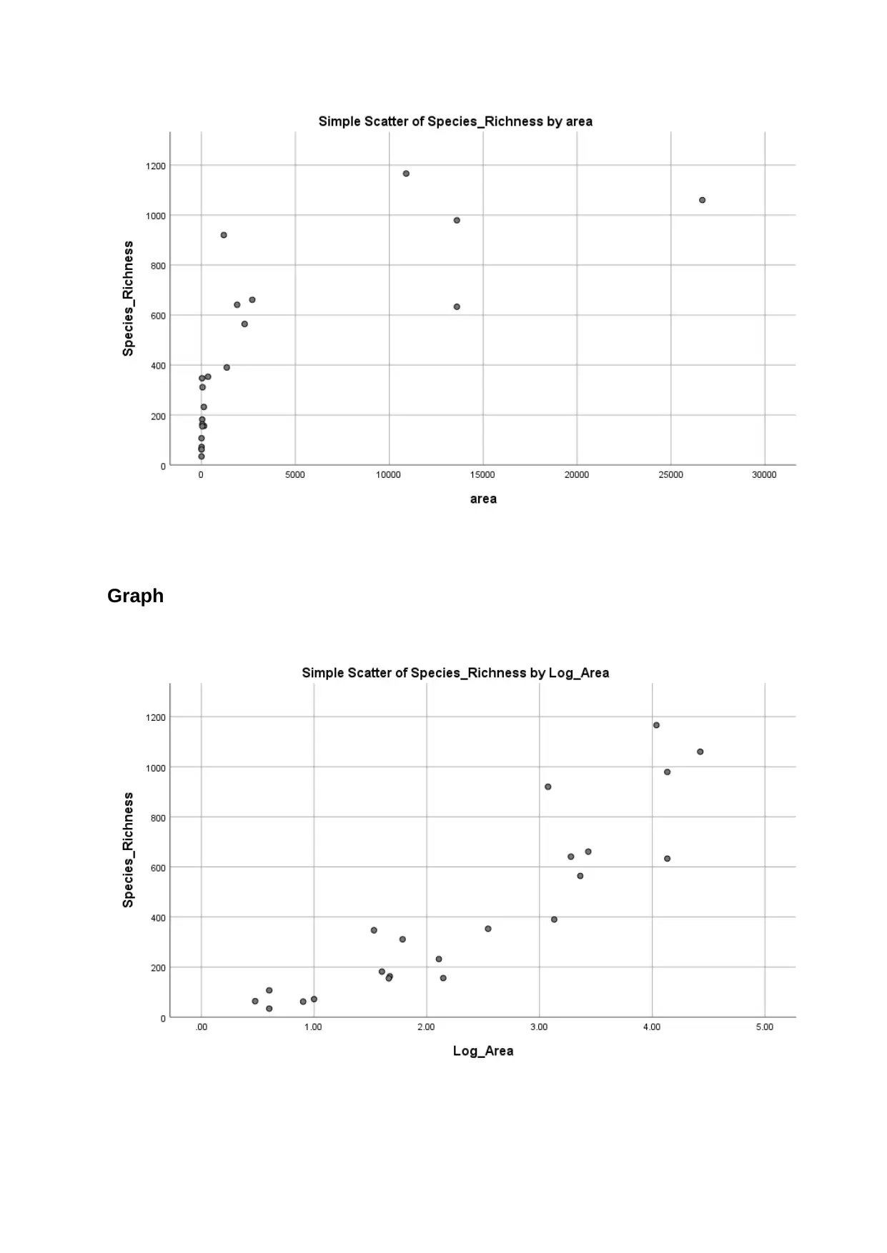
Graph
Graph
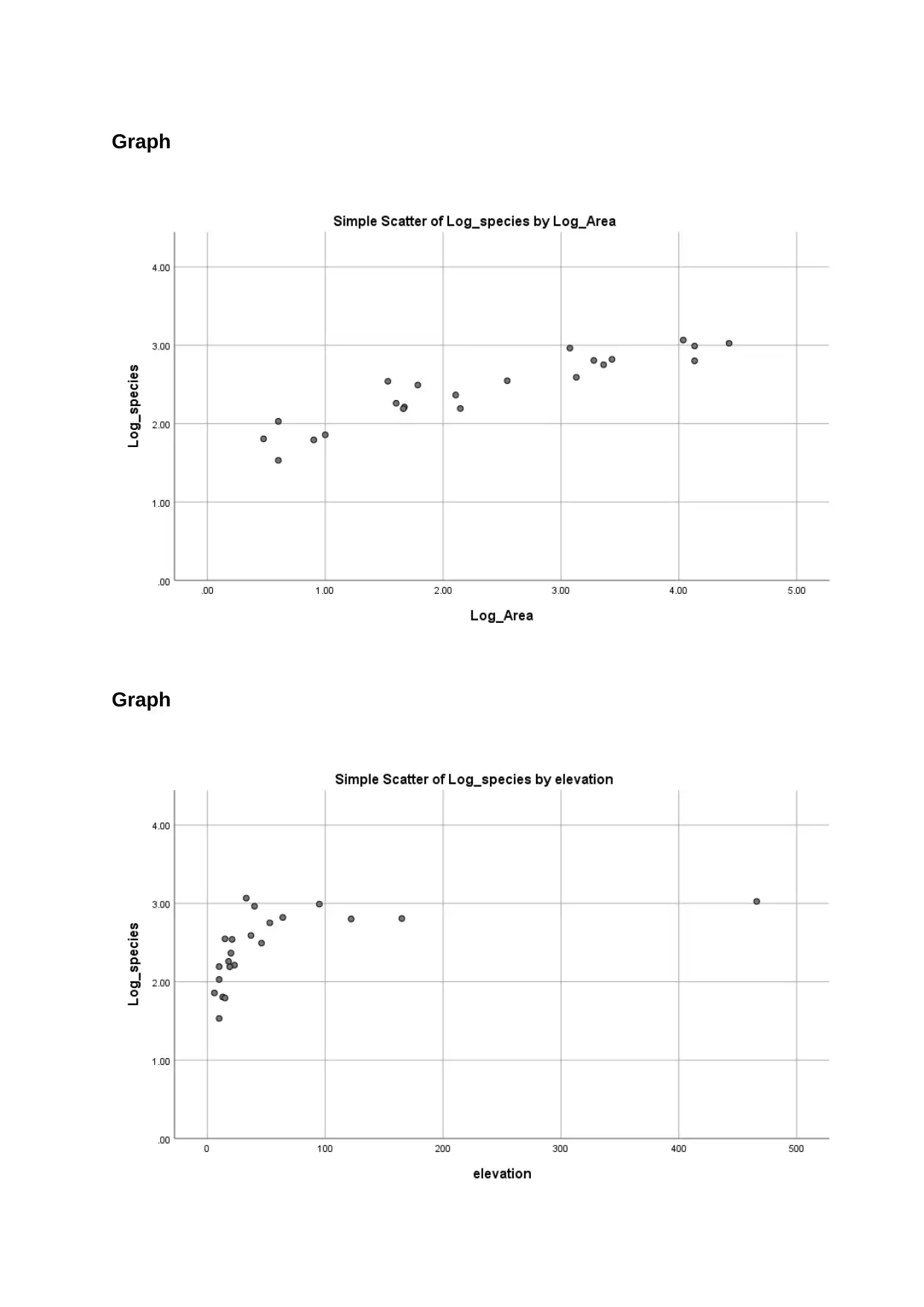
Graph
Graph
Graph
Graph
Graph
Paraphrase This Document
Need a fresh take? Get an instant paraphrase of this document with our AI Paraphraser
Graph
Graph
Explore
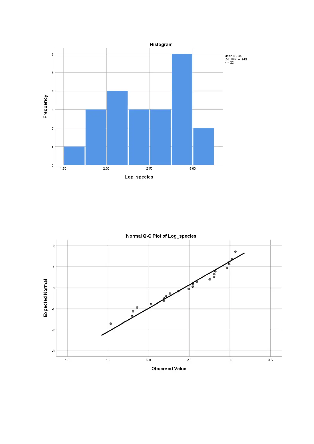
Log_species
Explore
Log_species
Secure Best Marks with AI Grader
Need help grading? Try our AI Grader for instant feedback on your assignments.
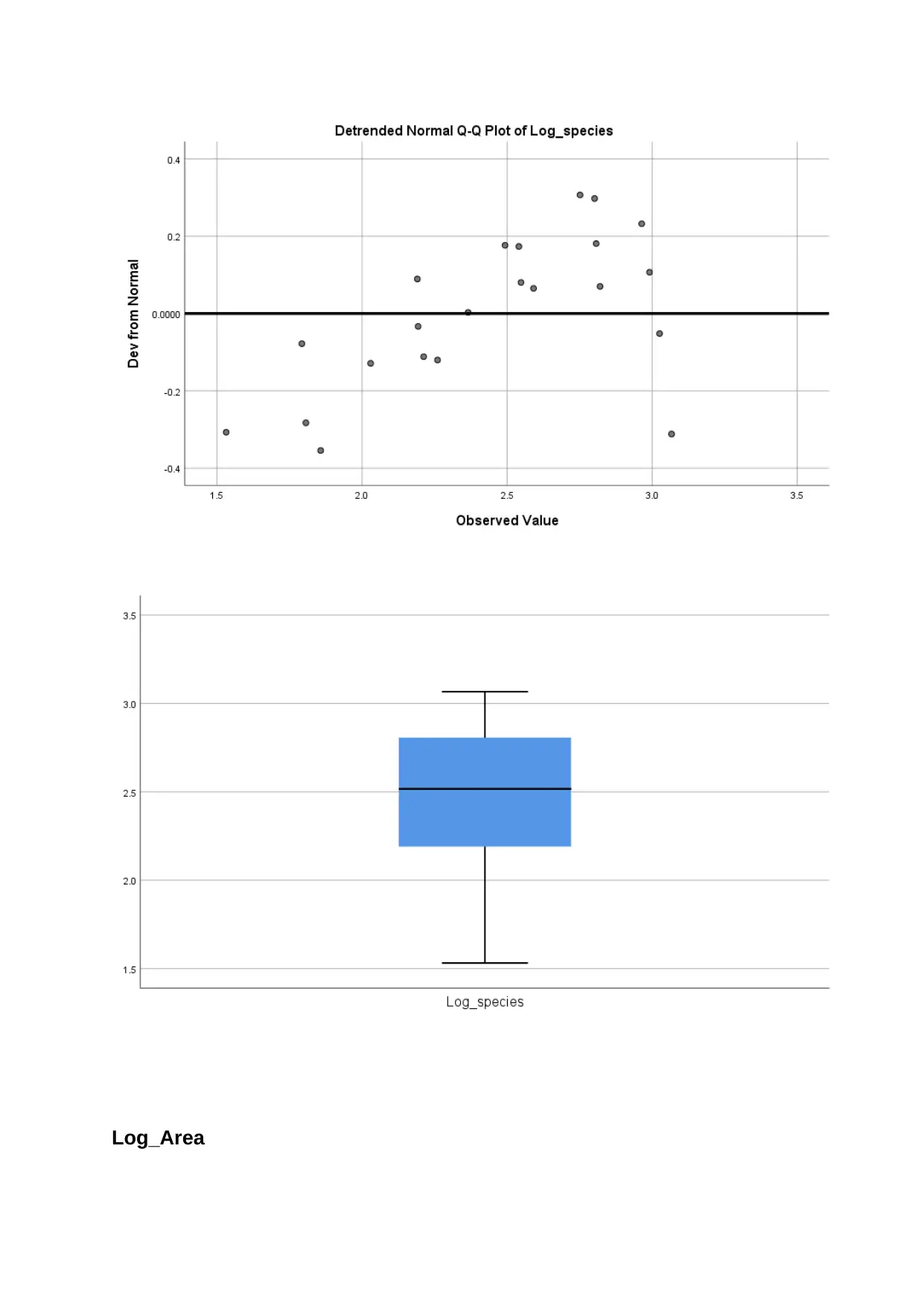
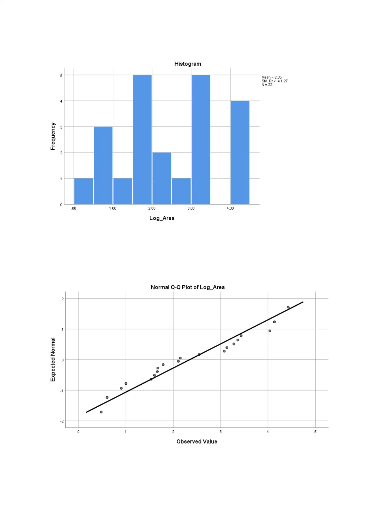
Log_Area
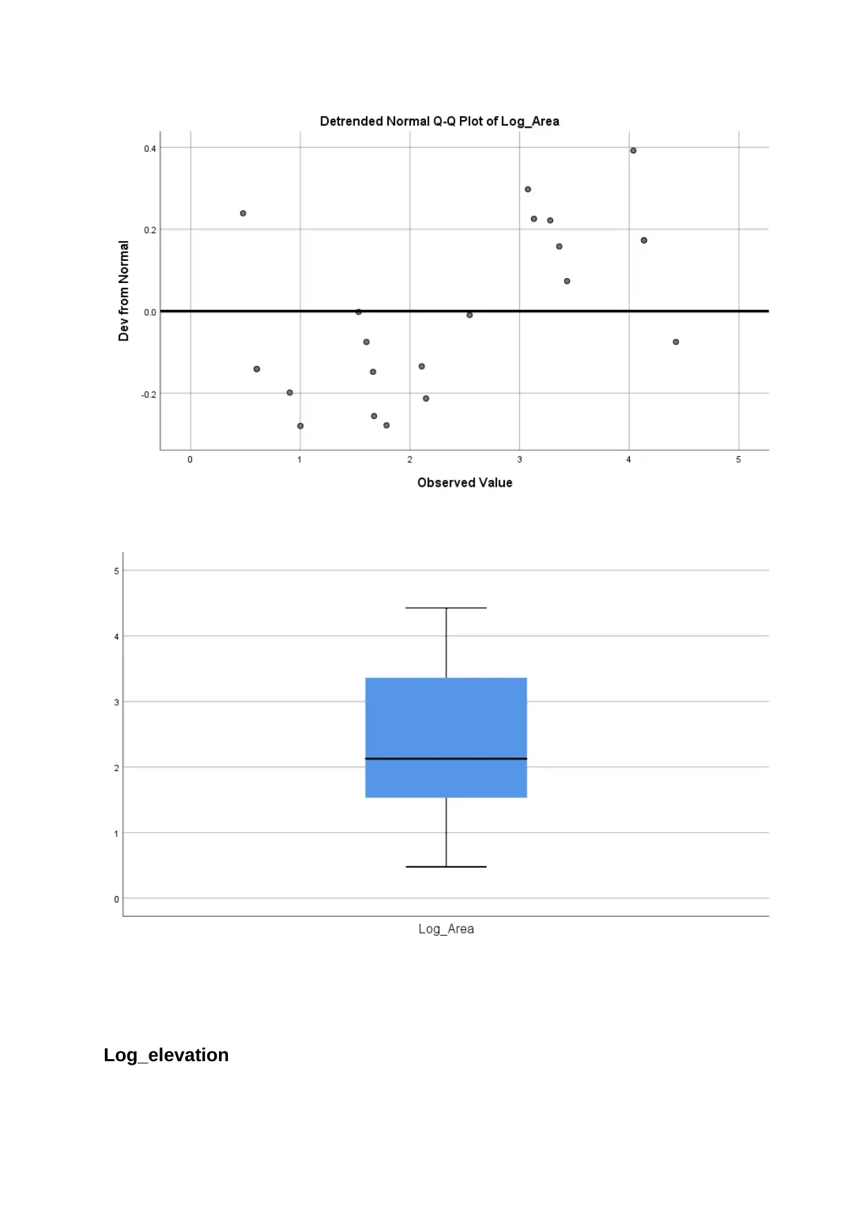
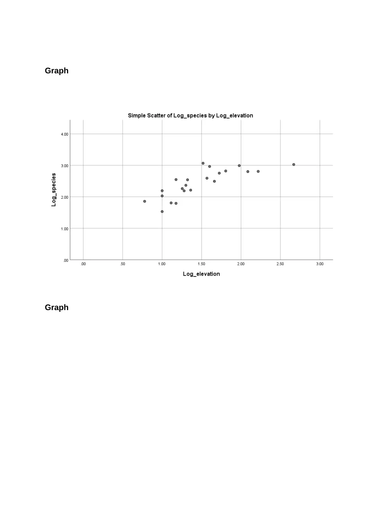
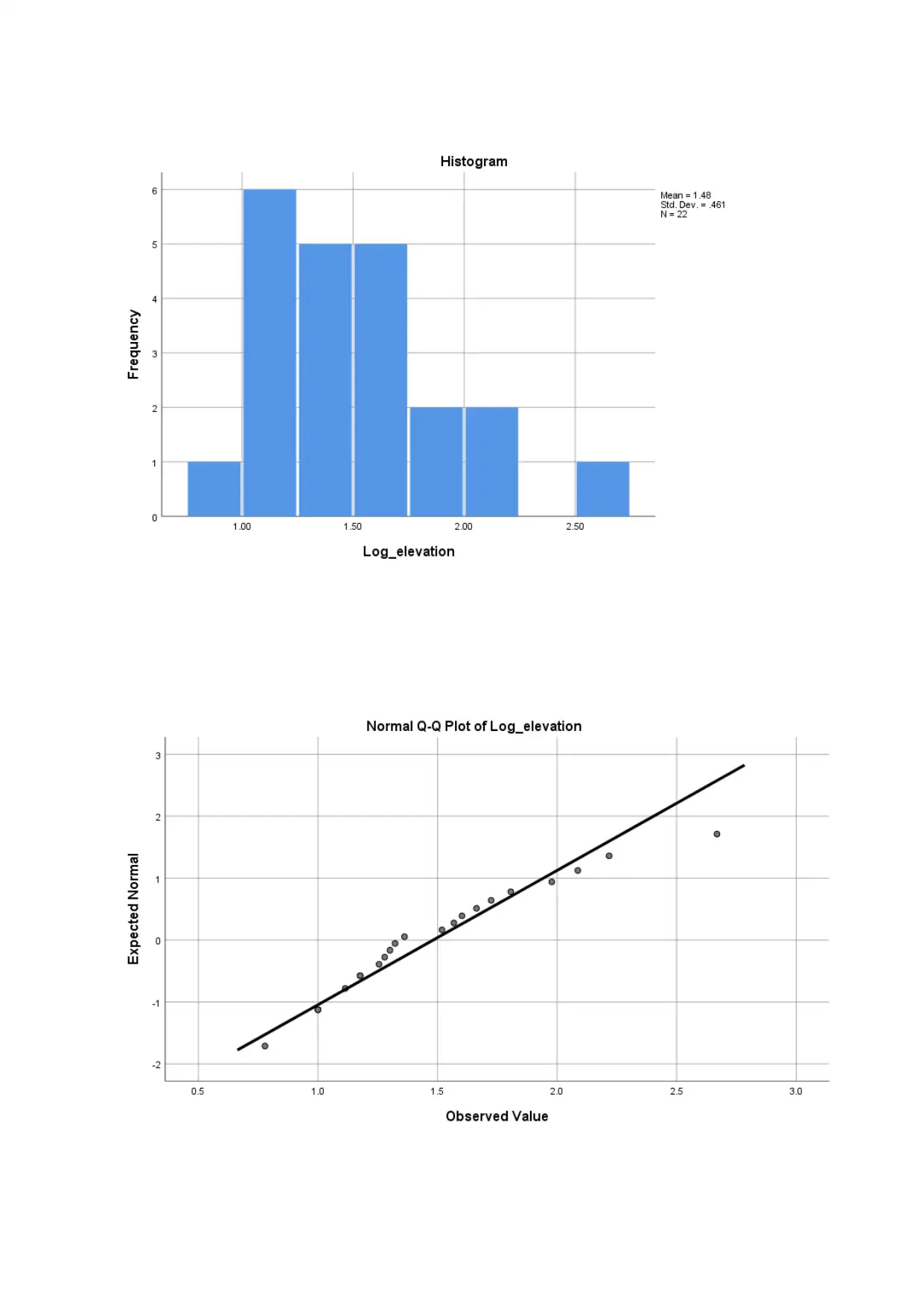
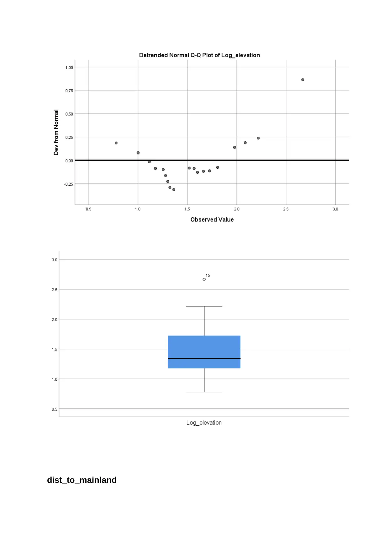
Log_elevation
Paraphrase This Document
Need a fresh take? Get an instant paraphrase of this document with our AI Paraphraser
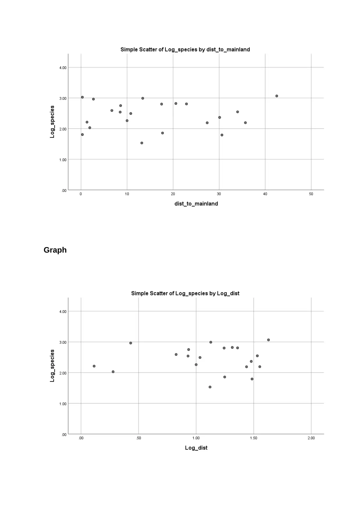
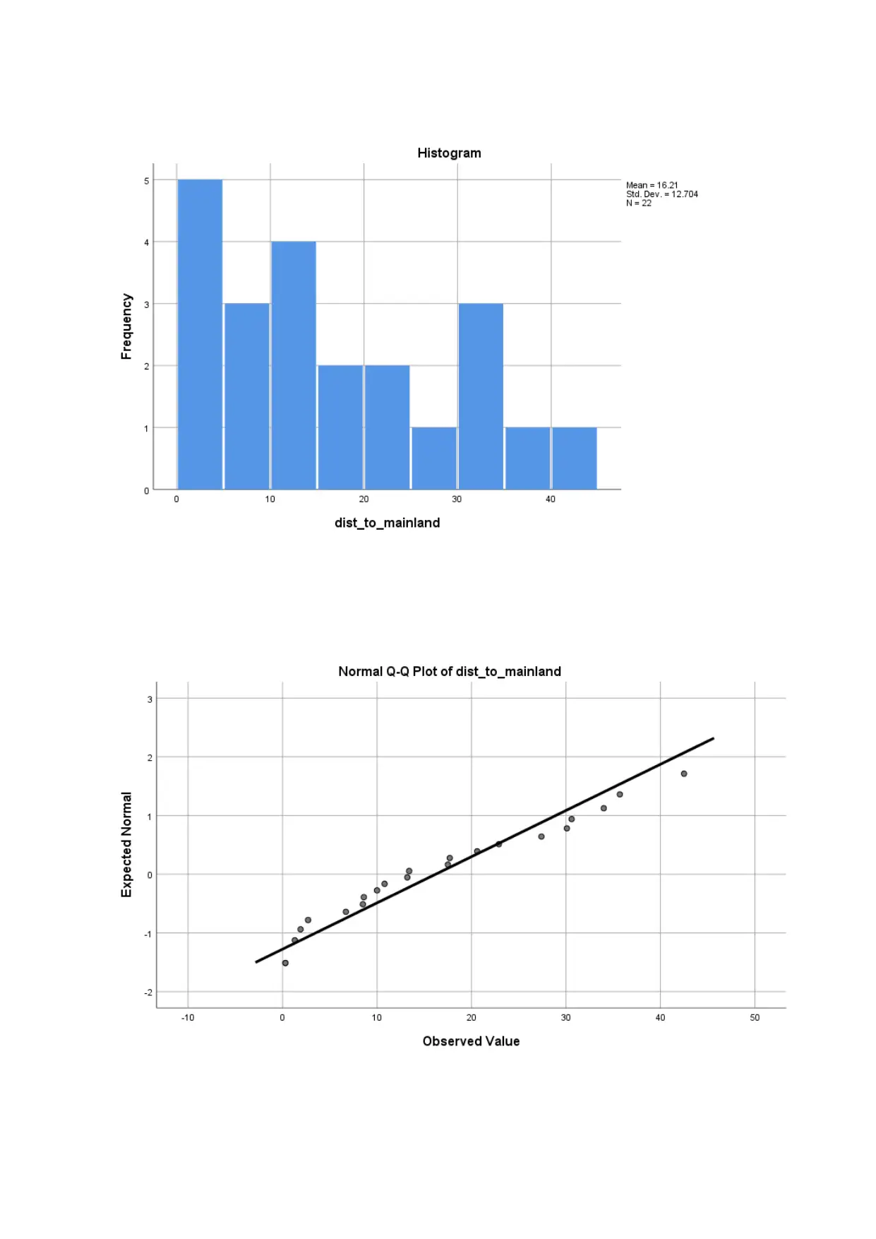
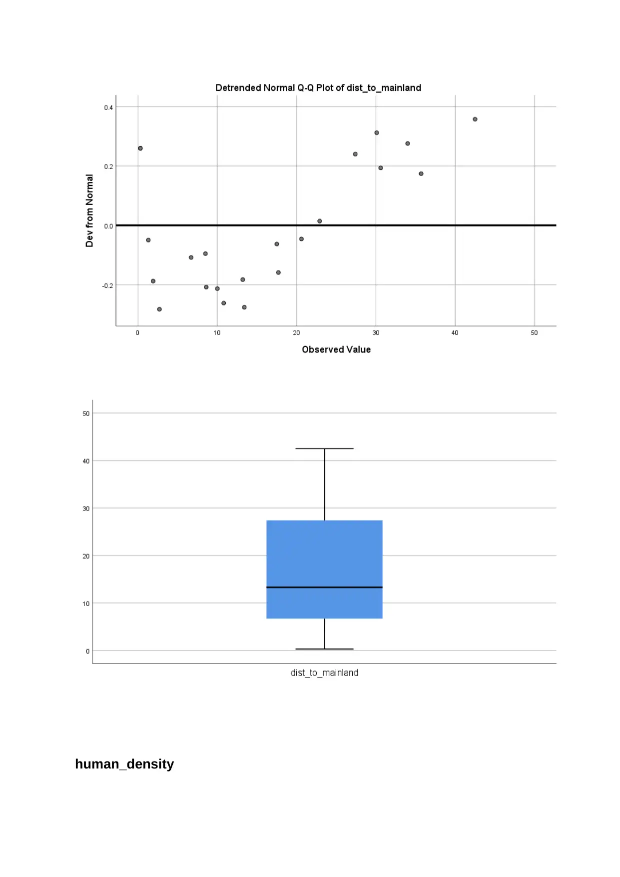
dist_to_mainland
Secure Best Marks with AI Grader
Need help grading? Try our AI Grader for instant feedback on your assignments.
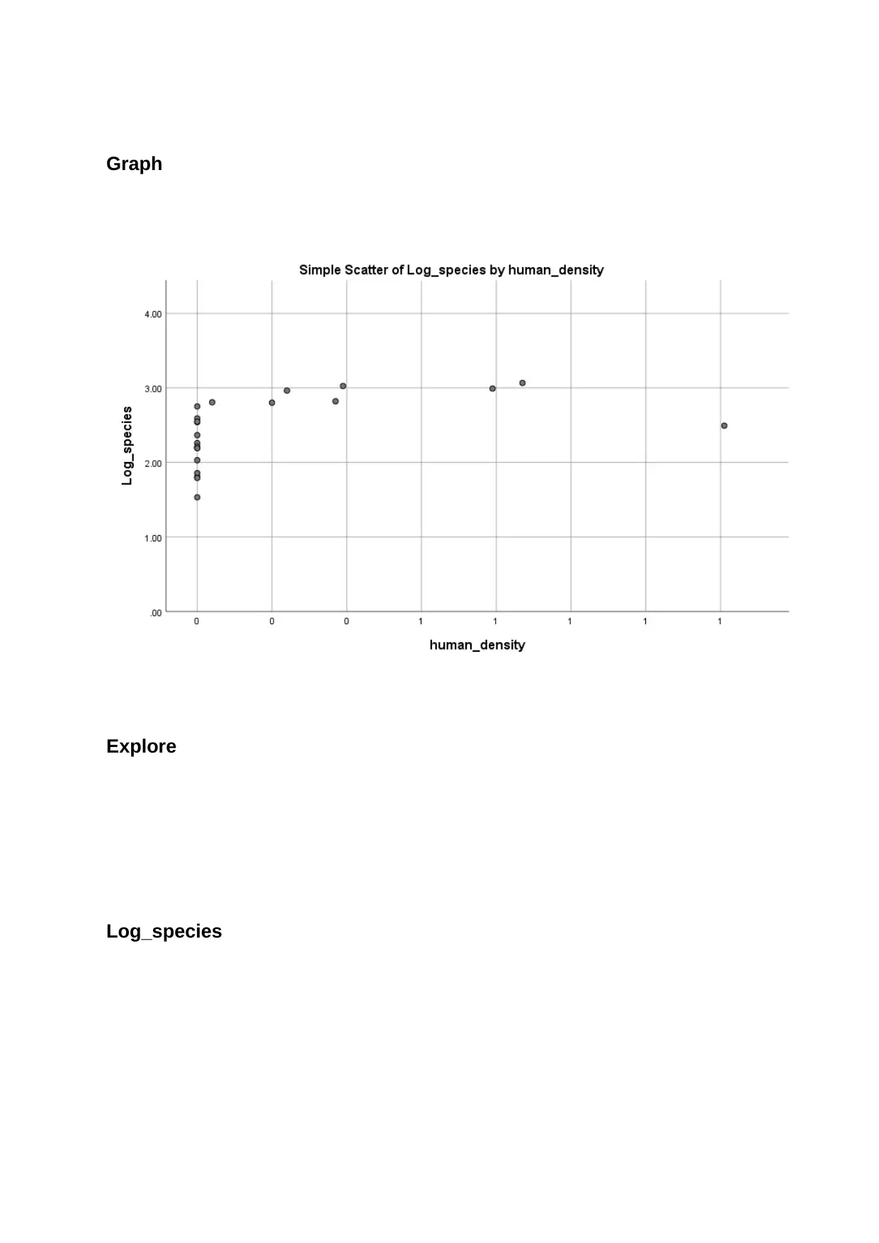
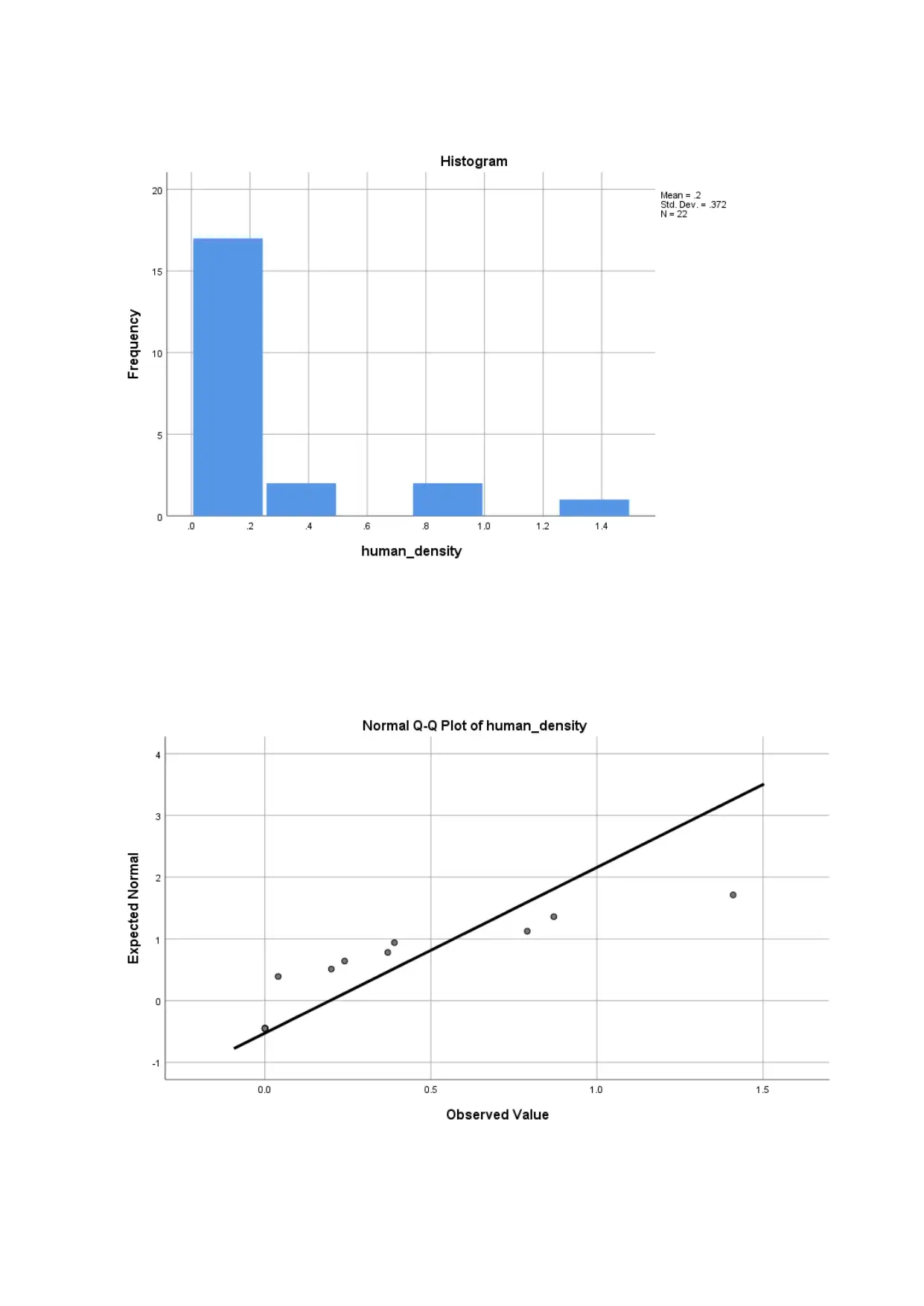
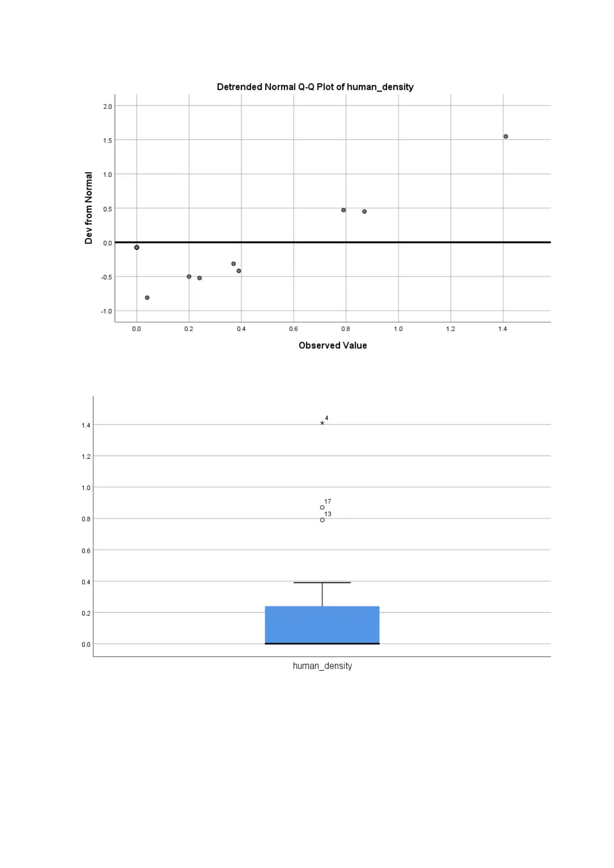
human_density
Paraphrase This Document
Need a fresh take? Get an instant paraphrase of this document with our AI Paraphraser
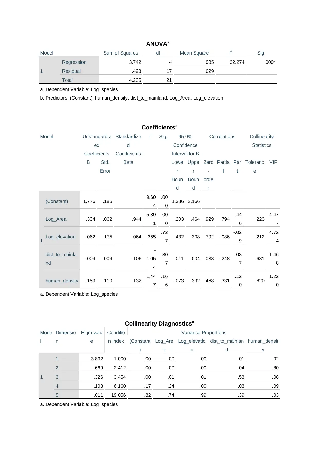
ANOVAa
Model Sum of Squares df Mean Square F Sig.
1
Regression 3.742 4 .935 32.274 .000b
Residual .493 17 .029
Total 4.235 21
a. Dependent Variable: Log_species
b. Predictors: (Constant), human_density, dist_to_mainland, Log_Area, Log_elevation
Coefficientsa
Model Unstandardiz
ed
Coefficients
Standardize
d
Coefficients
t Sig. 95.0%
Confidence
Interval for B
Correlations Collinearity
Statistics
B Std.
Error
Beta Lowe
r
Boun
d
Uppe
r
Boun
d
Zero
-
orde
r
Partia
l
Par
t
Toleranc
e
VIF
1
(Constant) 1.776 .185 9.60
4
.00
0 1.386 2.166
Log_Area .334 .062 .944 5.39
1
.00
0 .203 .464 .929 .794 .44
6 .223 4.47
7
Log_elevation -.062 .175 -.064 -.355 .72
7 -.432 .308 .792 -.086 -.02
9 .212 4.72
4
dist_to_mainla
nd -.004 .004 -.106
-
1.05
4
.30
7 -.011 .004 .038 -.248 -.08
7 .681 1.46
8
human_density .159 .110 .132 1.44
7
.16
6 -.073 .392 .468 .331 .12
0 .820 1.22
0
a. Dependent Variable: Log_species
Collinearity Diagnosticsa
Mode
l
Dimensio
n
Eigenvalu
e
Conditio
n Index
Variance Proportions
(Constant
)
Log_Are
a
Log_elevatio
n
dist_to_mainlan
d
human_densit
y
1
1 3.892 1.000 .00 .00 .00 .01 .02
2 .669 2.412 .00 .00 .00 .04 .80
3 .326 3.454 .00 .01 .01 .53 .08
4 .103 6.160 .17 .24 .00 .03 .09
5 .011 19.056 .82 .74 .99 .39 .03
a. Dependent Variable: Log_species
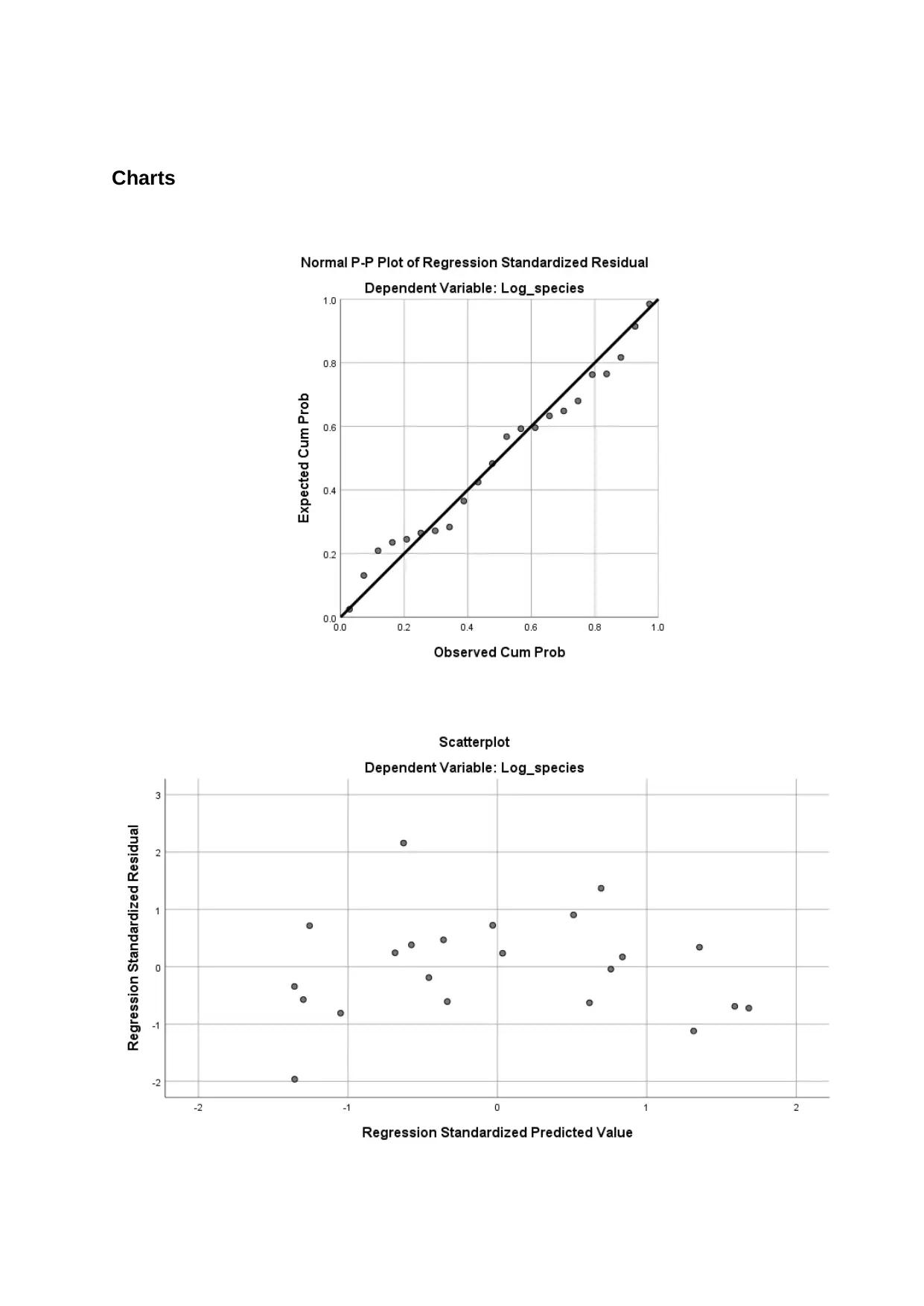
Charts
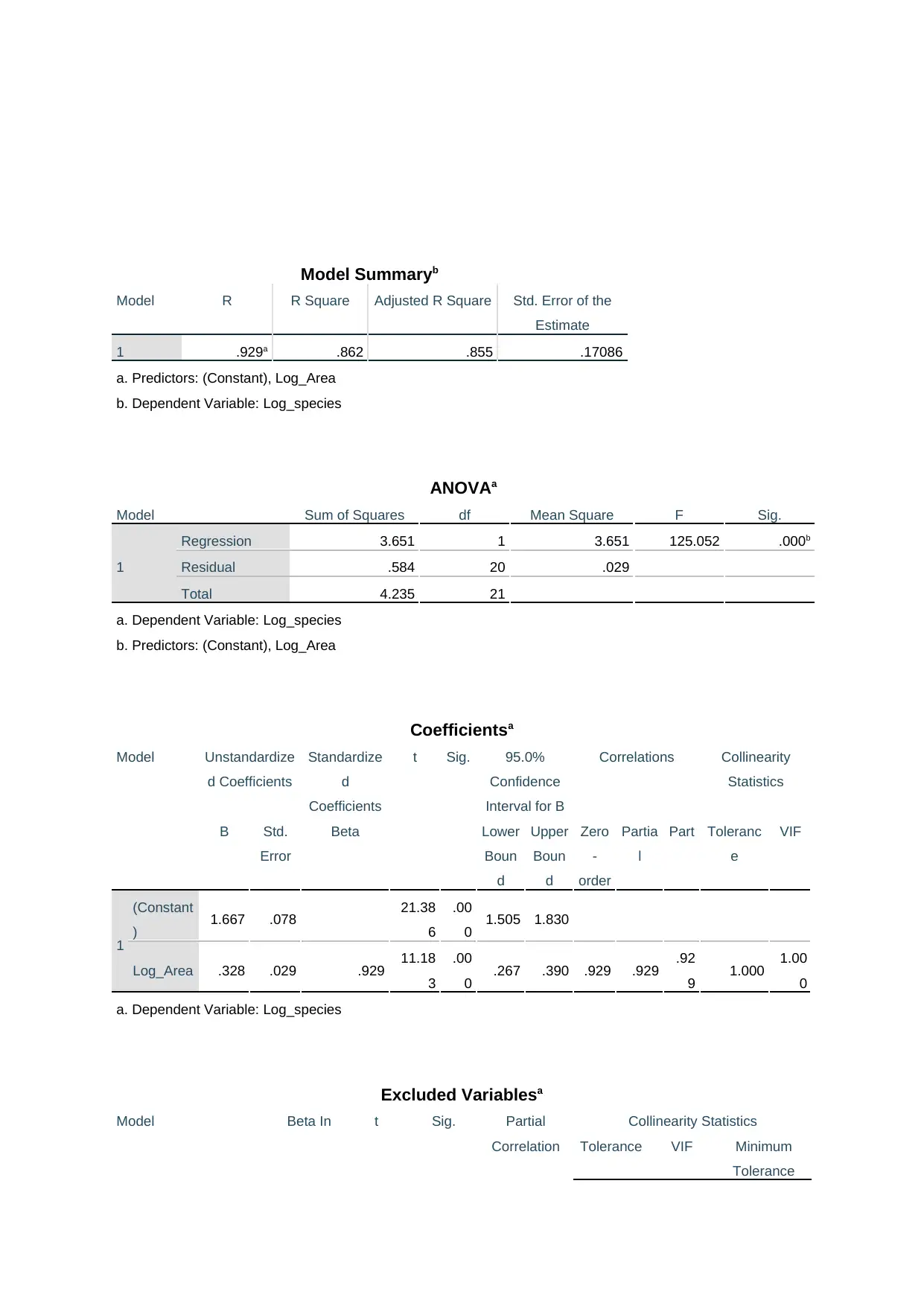
Model Summaryb
Model R R Square Adjusted R Square Std. Error of the
Estimate
1 .929a .862 .855 .17086
a. Predictors: (Constant), Log_Area
b. Dependent Variable: Log_species
ANOVAa
Model Sum of Squares df Mean Square F Sig.
1
Regression 3.651 1 3.651 125.052 .000b
Residual .584 20 .029
Total 4.235 21
a. Dependent Variable: Log_species
b. Predictors: (Constant), Log_Area
Coefficientsa
Model Unstandardize
d Coefficients
Standardize
d
Coefficients
t Sig. 95.0%
Confidence
Interval for B
Correlations Collinearity
Statistics
B Std.
Error
Beta Lower
Boun
d
Upper
Boun
d
Zero
-
order
Partia
l
Part Toleranc
e
VIF
1
(Constant
) 1.667 .078 21.38
6
.00
0 1.505 1.830
Log_Area .328 .029 .929 11.18
3
.00
0 .267 .390 .929 .929 .92
9 1.000 1.00
0
a. Dependent Variable: Log_species
Excluded Variablesa
Model Beta In t Sig. Partial
Correlation
Collinearity Statistics
Tolerance VIF Minimum
Tolerance
Secure Best Marks with AI Grader
Need help grading? Try our AI Grader for instant feedback on your assignments.
1
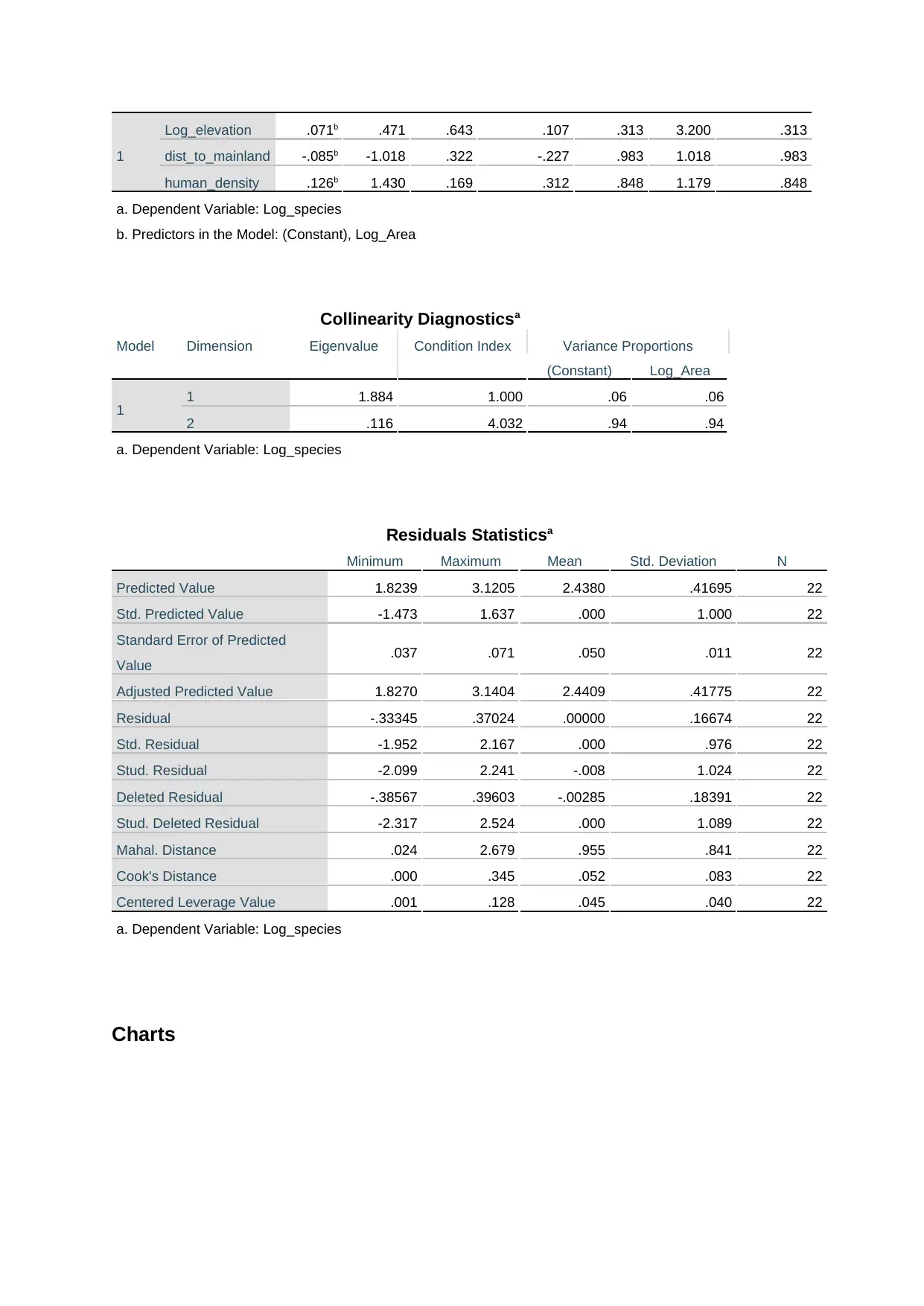
Log_elevation .071b .471 .643 .107 .313 3.200 .313
dist_to_mainland -.085b -1.018 .322 -.227 .983 1.018 .983
human_density .126b 1.430 .169 .312 .848 1.179 .848
a. Dependent Variable: Log_species
b. Predictors in the Model: (Constant), Log_Area
Collinearity Diagnosticsa
Model Dimension Eigenvalue Condition Index Variance Proportions
(Constant) Log_Area
1 1 1.884 1.000 .06 .06
2 .116 4.032 .94 .94
a. Dependent Variable: Log_species
Residuals Statisticsa
Minimum Maximum Mean Std. Deviation N
Predicted Value 1.8239 3.1205 2.4380 .41695 22
Std. Predicted Value -1.473 1.637 .000 1.000 22
Standard Error of Predicted
Value .037 .071 .050 .011 22
Adjusted Predicted Value 1.8270 3.1404 2.4409 .41775 22
Residual -.33345 .37024 .00000 .16674 22
Std. Residual -1.952 2.167 .000 .976 22
Stud. Residual -2.099 2.241 -.008 1.024 22
Deleted Residual -.38567 .39603 -.00285 .18391 22
Stud. Deleted Residual -2.317 2.524 .000 1.089 22
Mahal. Distance .024 2.679 .955 .841 22
Cook's Distance .000 .345 .052 .083 22
Centered Leverage Value .001 .128 .045 .040 22
a. Dependent Variable: Log_species
Charts
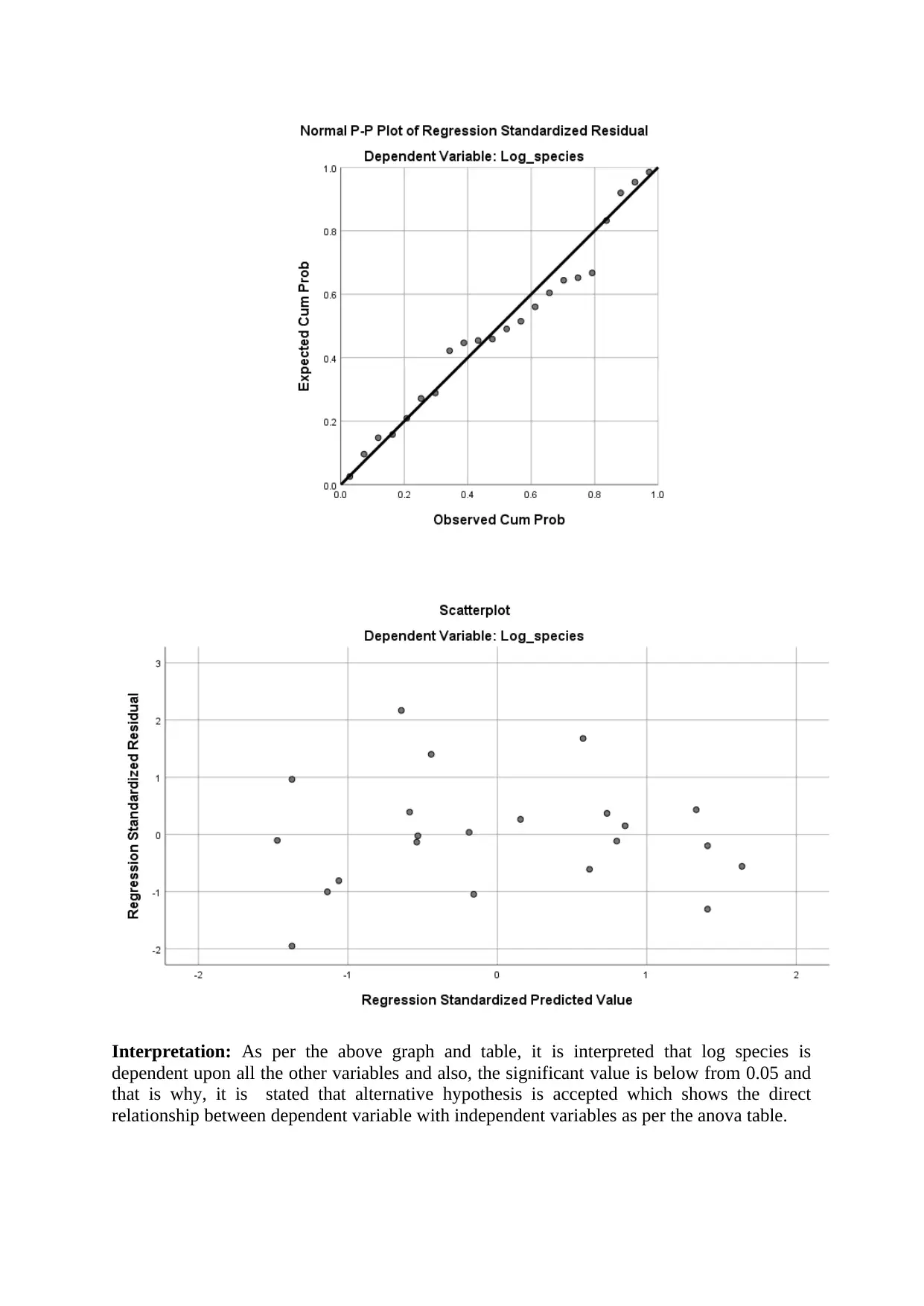
Interpretation: As per the above graph and table, it is interpreted that log species is
dependent upon all the other variables and also, the significant value is below from 0.05 and
that is why, it is stated that alternative hypothesis is accepted which shows the direct
relationship between dependent variable with independent variables as per the anova table.
dependent upon all the other variables and also, the significant value is below from 0.05 and
that is why, it is stated that alternative hypothesis is accepted which shows the direct
relationship between dependent variable with independent variables as per the anova table.
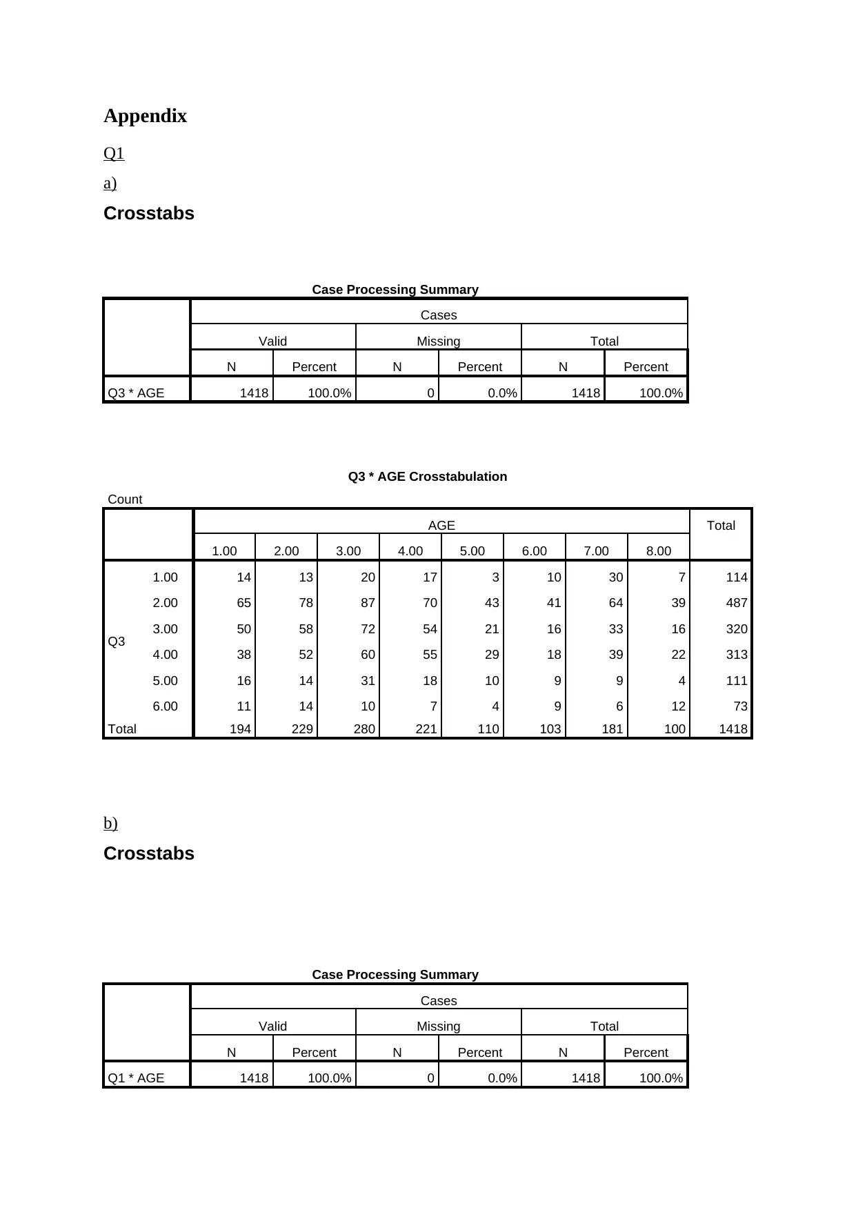
Appendix
Q1
a)
Crosstabs
Case Processing Summary
Cases
Valid Missing Total
N Percent N Percent N Percent
Q3 * AGE 1418 100.0% 0 0.0% 1418 100.0%
Q3 * AGE Crosstabulation
Count
AGE Total
1.00 2.00 3.00 4.00 5.00 6.00 7.00 8.00
Q3
1.00 14 13 20 17 3 10 30 7 114
2.00 65 78 87 70 43 41 64 39 487
3.00 50 58 72 54 21 16 33 16 320
4.00 38 52 60 55 29 18 39 22 313
5.00 16 14 31 18 10 9 9 4 111
6.00 11 14 10 7 4 9 6 12 73
Total 194 229 280 221 110 103 181 100 1418
b)
Crosstabs
Case Processing Summary
Cases
Valid Missing Total
N Percent N Percent N Percent
Q1 * AGE 1418 100.0% 0 0.0% 1418 100.0%
Paraphrase This Document
Need a fresh take? Get an instant paraphrase of this document with our AI Paraphraser
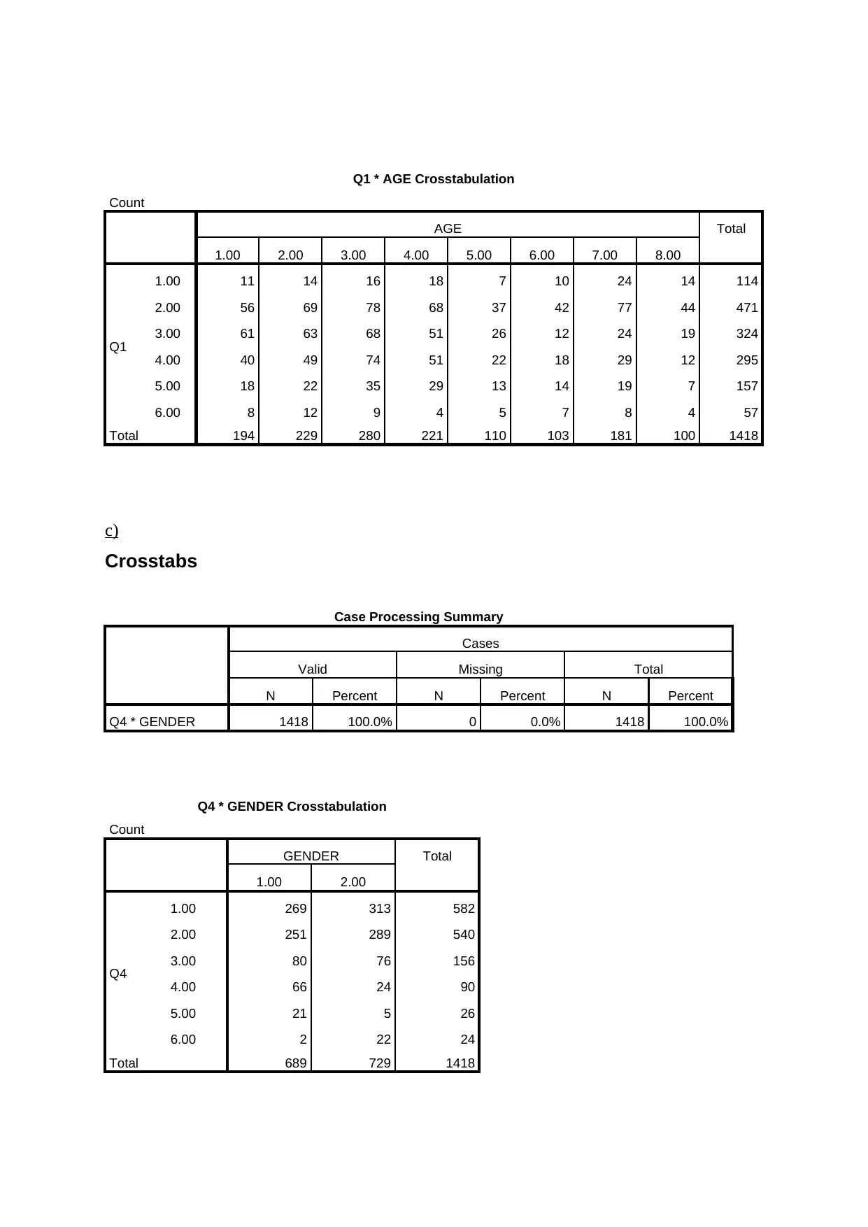
Q1 * AGE Crosstabulation
Count
AGE Total
1.00 2.00 3.00 4.00 5.00 6.00 7.00 8.00
Q1
1.00 11 14 16 18 7 10 24 14 114
2.00 56 69 78 68 37 42 77 44 471
3.00 61 63 68 51 26 12 24 19 324
4.00 40 49 74 51 22 18 29 12 295
5.00 18 22 35 29 13 14 19 7 157
6.00 8 12 9 4 5 7 8 4 57
Total 194 229 280 221 110 103 181 100 1418
c)
Crosstabs
Case Processing Summary
Cases
Valid Missing Total
N Percent N Percent N Percent
Q4 * GENDER 1418 100.0% 0 0.0% 1418 100.0%
Q4 * GENDER Crosstabulation
Count
GENDER Total
1.00 2.00
Q4
1.00 269 313 582
2.00 251 289 540
3.00 80 76 156
4.00 66 24 90
5.00 21 5 26
6.00 2 22 24
Total 689 729 1418
Count
AGE Total
1.00 2.00 3.00 4.00 5.00 6.00 7.00 8.00
Q1
1.00 11 14 16 18 7 10 24 14 114
2.00 56 69 78 68 37 42 77 44 471
3.00 61 63 68 51 26 12 24 19 324
4.00 40 49 74 51 22 18 29 12 295
5.00 18 22 35 29 13 14 19 7 157
6.00 8 12 9 4 5 7 8 4 57
Total 194 229 280 221 110 103 181 100 1418
c)
Crosstabs
Case Processing Summary
Cases
Valid Missing Total
N Percent N Percent N Percent
Q4 * GENDER 1418 100.0% 0 0.0% 1418 100.0%
Q4 * GENDER Crosstabulation
Count
GENDER Total
1.00 2.00
Q4
1.00 269 313 582
2.00 251 289 540
3.00 80 76 156
4.00 66 24 90
5.00 21 5 26
6.00 2 22 24
Total 689 729 1418
d)
Crosstabs
Case Processing Summary
Cases
Valid Missing Total
N Percent N Percent N Percent
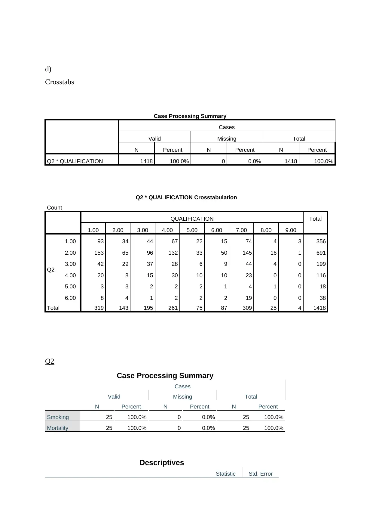
Q2 * QUALIFICATION 1418 100.0% 0 0.0% 1418 100.0%
Q2 * QUALIFICATION Crosstabulation
Count
QUALIFICATION Total
1.00 2.00 3.00 4.00 5.00 6.00 7.00 8.00 9.00
Q2
1.00 93 34 44 67 22 15 74 4 3 356
2.00 153 65 96 132 33 50 145 16 1 691
3.00 42 29 37 28 6 9 44 4 0 199
4.00 20 8 15 30 10 10 23 0 0 116
5.00 3 3 2 2 2 1 4 1 0 18
6.00 8 4 1 2 2 2 19 0 0 38
Total 319 143 195 261 75 87 309 25 4 1418
Q2
Case Processing Summary
Cases
Valid Missing Total
N Percent N Percent N Percent
Smoking 25 100.0% 0 0.0% 25 100.0%
Mortality 25 100.0% 0 0.0% 25 100.0%
Descriptives
Statistic Std. Error
Crosstabs
Case Processing Summary
Cases
Valid Missing Total
N Percent N Percent N Percent
Q2 * QUALIFICATION 1418 100.0% 0 0.0% 1418 100.0%
Q2 * QUALIFICATION Crosstabulation
Count
QUALIFICATION Total
1.00 2.00 3.00 4.00 5.00 6.00 7.00 8.00 9.00
Q2
1.00 93 34 44 67 22 15 74 4 3 356
2.00 153 65 96 132 33 50 145 16 1 691
3.00 42 29 37 28 6 9 44 4 0 199
4.00 20 8 15 30 10 10 23 0 0 116
5.00 3 3 2 2 2 1 4 1 0 18
6.00 8 4 1 2 2 2 19 0 0 38
Total 319 143 195 261 75 87 309 25 4 1418
Q2
Case Processing Summary
Cases
Valid Missing Total
N Percent N Percent N Percent
Smoking 25 100.0% 0 0.0% 25 100.0%
Mortality 25 100.0% 0 0.0% 25 100.0%
Descriptives
Statistic Std. Error
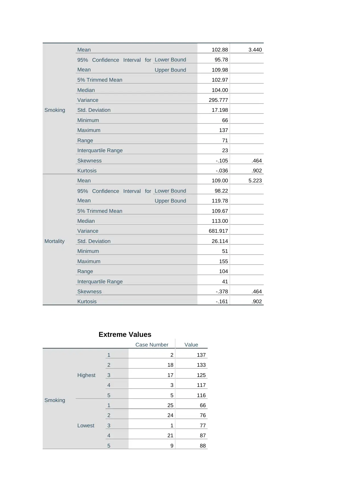
Smoking
Mean 102.88 3.440
95% Confidence Interval for
Mean
Lower Bound 95.78
Upper Bound 109.98
5% Trimmed Mean 102.97
Median 104.00
Variance 295.777
Std. Deviation 17.198
Minimum 66
Maximum 137
Range 71
Interquartile Range 23
Skewness -.105 .464
Kurtosis -.036 .902
Mortality
Mean 109.00 5.223
95% Confidence Interval for
Mean
Lower Bound 98.22
Upper Bound 119.78
5% Trimmed Mean 109.67
Median 113.00
Variance 681.917
Std. Deviation 26.114
Minimum 51
Maximum 155
Range 104
Interquartile Range 41
Skewness -.378 .464
Kurtosis -.161 .902
Extreme Values
Case Number Value
Smoking
Highest
1 2 137
2 18 133
3 17 125
4 3 117
5 5 116
Lowest
1 25 66
2 24 76
3 1 77
4 21 87
5 9 88
Secure Best Marks with AI Grader
Need help grading? Try our AI Grader for instant feedback on your assignments.
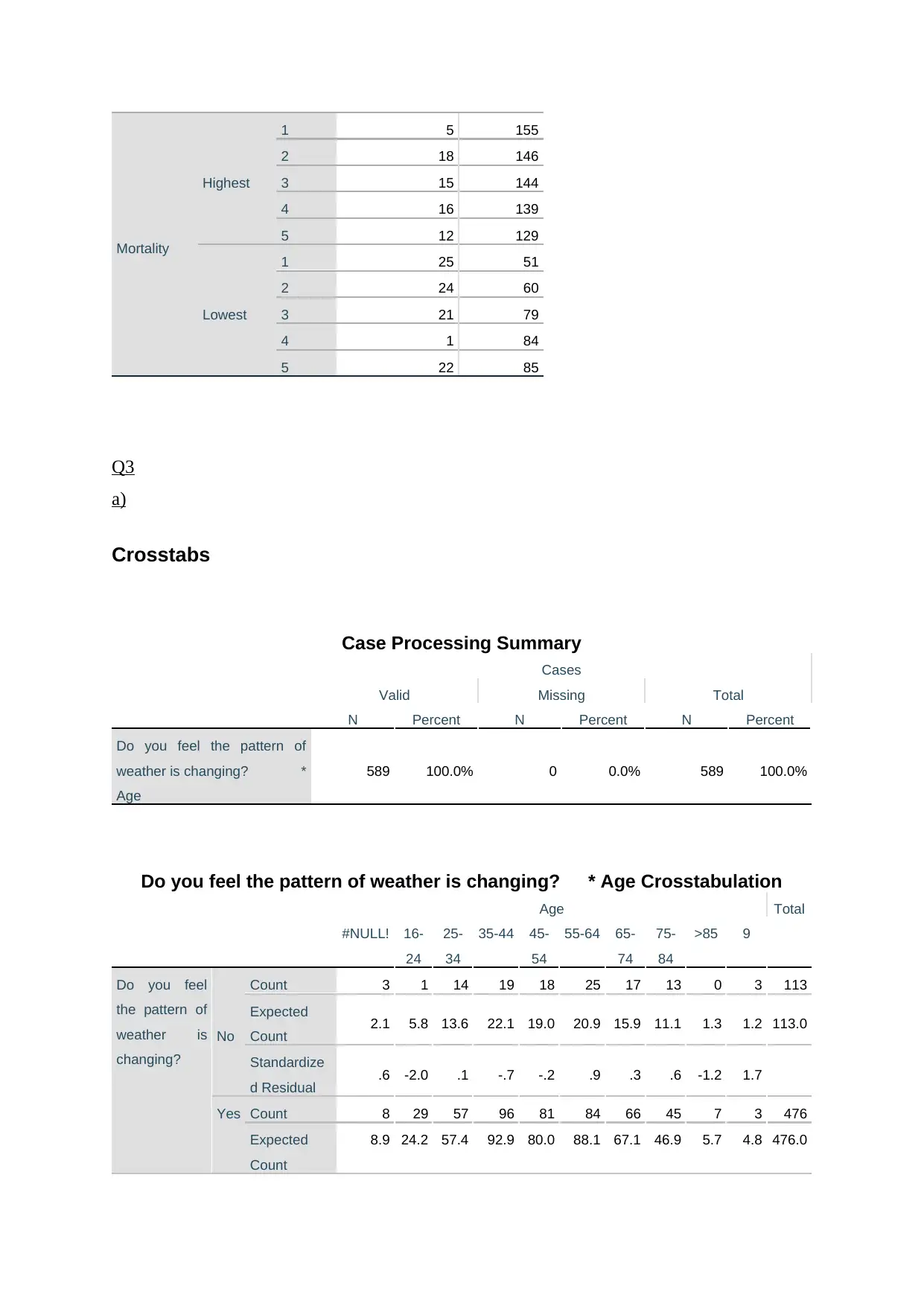
Mortality
Highest
1 5 155
2 18 146
3 15 144
4 16 139
5 12 129
Lowest
1 25 51
2 24 60
3 21 79
4 1 84
5 22 85
Q3
a)
Crosstabs
Case Processing Summary
Cases
Valid Missing Total
N Percent N Percent N Percent
Do you feel the pattern of
weather is changing? *
Age
589 100.0% 0 0.0% 589 100.0%
Do you feel the pattern of weather is changing? * Age Crosstabulation
Age Total
#NULL! 16-
24
25-
34
35-44 45-
54
55-64 65-
74
75-
84
>85 9
Do you feel
the pattern of
weather is
changing?
No
Count 3 1 14 19 18 25 17 13 0 3 113
Expected
Count 2.1 5.8 13.6 22.1 19.0 20.9 15.9 11.1 1.3 1.2 113.0
Standardize
d Residual .6 -2.0 .1 -.7 -.2 .9 .3 .6 -1.2 1.7
Yes Count 8 29 57 96 81 84 66 45 7 3 476
Expected
Count
8.9 24.2 57.4 92.9 80.0 88.1 67.1 46.9 5.7 4.8 476.0
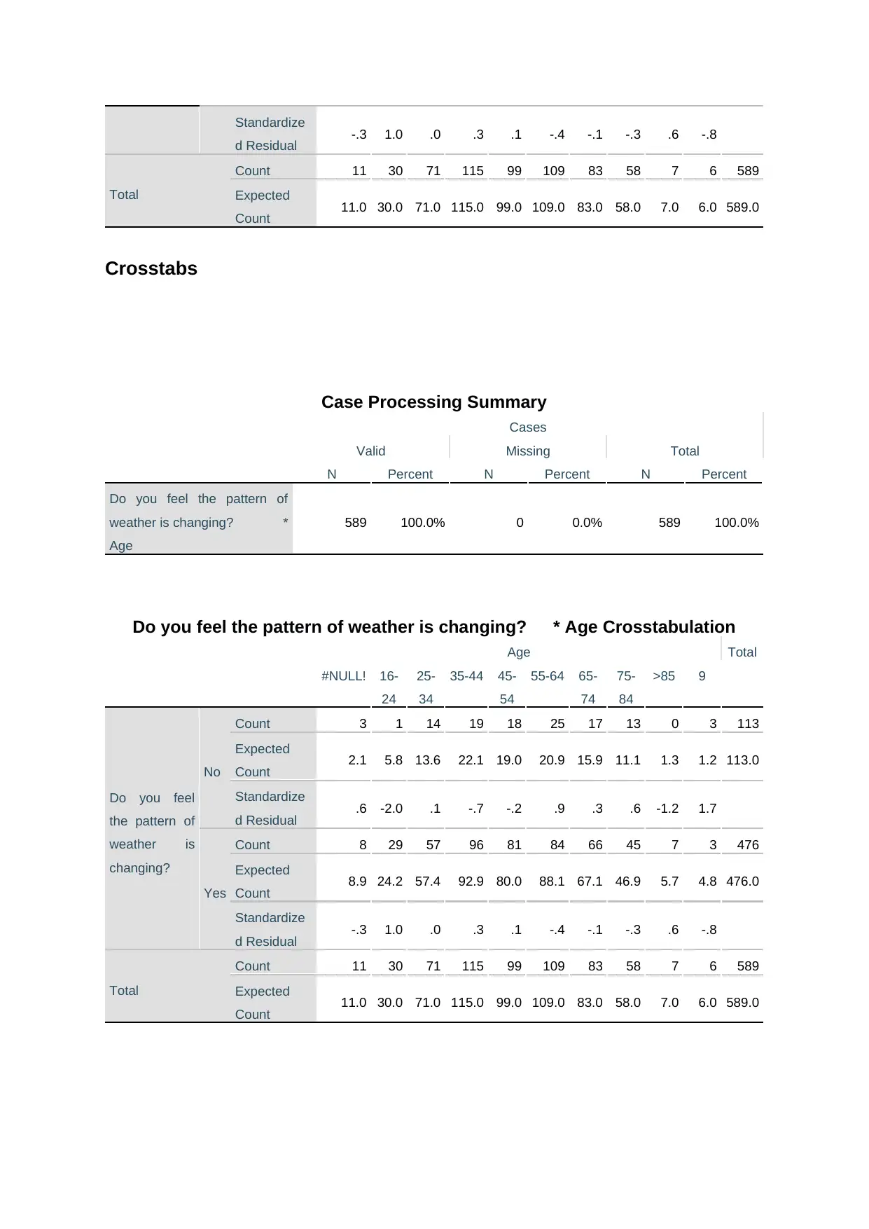
Standardize
d Residual -.3 1.0 .0 .3 .1 -.4 -.1 -.3 .6 -.8
Total
Count 11 30 71 115 99 109 83 58 7 6 589
Expected
Count 11.0 30.0 71.0 115.0 99.0 109.0 83.0 58.0 7.0 6.0 589.0
Crosstabs
Case Processing Summary
Cases
Valid Missing Total
N Percent N Percent N Percent
Do you feel the pattern of
weather is changing? *
Age
589 100.0% 0 0.0% 589 100.0%
Do you feel the pattern of weather is changing? * Age Crosstabulation
Age Total
#NULL! 16-
24
25-
34
35-44 45-
54
55-64 65-
74
75-
84
>85 9
Do you feel
the pattern of
weather is
changing?
No
Count 3 1 14 19 18 25 17 13 0 3 113
Expected
Count 2.1 5.8 13.6 22.1 19.0 20.9 15.9 11.1 1.3 1.2 113.0
Standardize
d Residual .6 -2.0 .1 -.7 -.2 .9 .3 .6 -1.2 1.7
Yes
Count 8 29 57 96 81 84 66 45 7 3 476
Expected
Count 8.9 24.2 57.4 92.9 80.0 88.1 67.1 46.9 5.7 4.8 476.0
Standardize
d Residual -.3 1.0 .0 .3 .1 -.4 -.1 -.3 .6 -.8
Total
Count 11 30 71 115 99 109 83 58 7 6 589
Expected
Count 11.0 30.0 71.0 115.0 99.0 109.0 83.0 58.0 7.0 6.0 589.0
d Residual -.3 1.0 .0 .3 .1 -.4 -.1 -.3 .6 -.8
Total
Count 11 30 71 115 99 109 83 58 7 6 589
Expected
Count 11.0 30.0 71.0 115.0 99.0 109.0 83.0 58.0 7.0 6.0 589.0
Crosstabs
Case Processing Summary
Cases
Valid Missing Total
N Percent N Percent N Percent
Do you feel the pattern of
weather is changing? *
Age
589 100.0% 0 0.0% 589 100.0%
Do you feel the pattern of weather is changing? * Age Crosstabulation
Age Total
#NULL! 16-
24
25-
34
35-44 45-
54
55-64 65-
74
75-
84
>85 9
Do you feel
the pattern of
weather is
changing?
No
Count 3 1 14 19 18 25 17 13 0 3 113
Expected
Count 2.1 5.8 13.6 22.1 19.0 20.9 15.9 11.1 1.3 1.2 113.0
Standardize
d Residual .6 -2.0 .1 -.7 -.2 .9 .3 .6 -1.2 1.7
Yes
Count 8 29 57 96 81 84 66 45 7 3 476
Expected
Count 8.9 24.2 57.4 92.9 80.0 88.1 67.1 46.9 5.7 4.8 476.0
Standardize
d Residual -.3 1.0 .0 .3 .1 -.4 -.1 -.3 .6 -.8
Total
Count 11 30 71 115 99 109 83 58 7 6 589
Expected
Count 11.0 30.0 71.0 115.0 99.0 109.0 83.0 58.0 7.0 6.0 589.0
b)
Crosstabs
Case Processing Summary
Cases
Valid Missing Total
N Percent N Percent N Percent
Climate change is inevitable
because of the way modern
society works. * Highest
Qualification
589 100.0% 0 0.0% 589 100.0%
Climate change is inevitable because of the way modern society works. *
Highest Qualification Crosstabulation
Highest Qualification Total
#NULL
!
NON
E
GCS
E
A
LEVE
L
NV
Q
DEGRE
E
POSTGRA
D
OTHE
R
Climate
change
is
inevitabl
e
because
of the
way
modern
society
works.
#NULL!
Count 3 6 6 2 8 7 6 3 41
Expected
Count 1.2 6.0 5.1 5.9 3.5 10.2 6.6 2.6 41.0
Standardize
d Residual 1.7 .0 .4 -1.6 2.4 -1.0 -.2 .3
strongly
disagre
e
Count 0 1 2 6 1 5 4 2 21
Expected
Count .6 3.1 2.6 3.0 1.8 5.2 3.4 1.3 21.0
Standardize
d Residual -.8 -1.2 -.4 1.7 -.6 -.1 .3 .6
Disagre
e
Count 1 11 12 22 12 35 24 7 124
Expected
Count 3.6 18.1 15.4 17.9 10.5 30.7 20.0 7.8 124.
0
Standardize
d Residual -1.4 -1.7 -.9 1.0 .5 .8 .9 -.3
Neither
agree or
disagre
e
Count 1 19 10 9 5 31 22 3 100
Expected
Count 2.9 14.6 12.4 14.4 8.5 24.8 16.1 6.3 100.
0
Standardize
d Residual
-1.1 1.2 -.7 -1.4 -1.2 1.2 1.5 -1.3
Paraphrase This Document
Need a fresh take? Get an instant paraphrase of this document with our AI Paraphraser
Agree
Count 9 35 31 35 15 59 29 16 229
Expected
Count 6.6 33.4 28.4 33.0 19.4 56.8 36.9 14.4 229.
0
Standardize
d Residual .9 .3 .5 .3 -1.0 .3 -1.3 .4
Strongly
agree
Count 3 14 12 11 9 9 10 6 74
Expected
Count 2.1 10.8 9.2 10.7 6.3 18.3 11.9 4.6 74.0
Standardize
d Residual .6 1.0 .9 .1 1.1 -2.2 -.6 .6
Total
Count 17 86 73 85 50 146 95 37 589
Expected
Count 17.0 86.0 73.0 85.0 50.0 146.0 95.0 37.0 589.
0
Crosstabs
Case Processing Summary
Cases
Valid Missing Total
N Percent N Percent N Percent
Climate change is inevitable
because of the way modern
society works. * Highest
Qualification
589 100.0% 0 0.0% 589 100.0%
Climate change is inevitable because of the way modern society works. *
Highest Qualification Crosstabulation
Highest Qualification Total
#NULL
!
NON
E
GCS
E
A
LEVE
L
NV
Q
DEGRE
E
POSTGRA
D
OTHE
R
Climate
change
is
inevitabl
e
#NULL! Count 3 6 6 2 8 7 6 3 41
Expected
Count 1.2 6.0 5.1 5.9 3.5 10.2 6.6 2.6 41.0
Standardize
d Residual
1.7 .0 .4 -1.6 2.4 -1.0 -.2 .3
because
of the
way
modern
society
works.
strongly
disagre
e
Count 0 1 2 6 1 5 4 2 21
Expected
Count .6 3.1 2.6 3.0 1.8 5.2 3.4 1.3 21.0
Standardize
d Residual -.8 -1.2 -.4 1.7 -.6 -.1 .3 .6
Disagre
e
Count 1 11 12 22 12 35 24 7 124
Expected
Count 3.6 18.1 15.4 17.9 10.5 30.7 20.0 7.8 124.
0
Standardize
d Residual -1.4 -1.7 -.9 1.0 .5 .8 .9 -.3
Neither
agree or
disagre
e
Count 1 19 10 9 5 31 22 3 100
Expected
Count 2.9 14.6 12.4 14.4 8.5 24.8 16.1 6.3 100.
0
Standardize
d Residual -1.1 1.2 -.7 -1.4 -1.2 1.2 1.5 -1.3
Agree
Count 9 35 31 35 15 59 29 16 229
Expected
Count 6.6 33.4 28.4 33.0 19.4 56.8 36.9 14.4 229.
0
Standardize
d Residual .9 .3 .5 .3 -1.0 .3 -1.3 .4
Strongly
agree
Count 3 14 12 11 9 9 10 6 74
Expected
Count 2.1 10.8 9.2 10.7 6.3 18.3 11.9 4.6 74.0
Standardize
d Residual .6 1.0 .9 .1 1.1 -2.2 -.6 .6
Total
Count 17 86 73 85 50 146 95 37 589
Expected
Count 17.0 86.0 73.0 85.0 50.0 146.0 95.0 37.0 589.
0
c)
Crosstabs
Case Processing Summary
Cases
Valid Missing Total
N Percent N Percent N Percent
Do you think anything can be
done to tackle climate change
* Gender
589 100.0% 0 0.0% 589 100.0%
Do you think anything can be done to tackle climate change * Gender
Crosstabulation
Gender Total
Female Male
Do you think anything can be
done to tackle climate change
No
Count 120 90 210
Expected Count 114.1 95.9 210.0
Standardized Residual .6 -.6
Yes
Count 200 179 379
Expected Count 205.9 173.1 379.0
Standardized Residual -.4 .4
Total Count 320 269 589
Expected Count 320.0 269.0 589.0
d)
Crosstabs
Case Processing Summary
Cases
Valid Missing Total
N Percent N Percent N Percent
Have you experienced flood
damage? * Climate change is
just a natural fluctuation in
Earth’s temperatures
589 100.0% 0 0.0% 589 100.0%
Have you experienced flood damage? * Climate change is just a natural
fluctuation in Earth’s temperatures Crosstabulation
Climate change is just a natural fluctuation in Earth’s
temperatures
Total
#NULL! strongly
disagree
Disagree Neither
agree or
disagree
Agree Strongly
agree
No Count 33 39 152 134 59 23 440
Do you think anything can be
done to tackle climate change
* Gender
589 100.0% 0 0.0% 589 100.0%
Do you think anything can be done to tackle climate change * Gender
Crosstabulation
Gender Total
Female Male
Do you think anything can be
done to tackle climate change
No
Count 120 90 210
Expected Count 114.1 95.9 210.0
Standardized Residual .6 -.6
Yes
Count 200 179 379
Expected Count 205.9 173.1 379.0
Standardized Residual -.4 .4
Total Count 320 269 589
Expected Count 320.0 269.0 589.0
d)
Crosstabs
Case Processing Summary
Cases
Valid Missing Total
N Percent N Percent N Percent
Have you experienced flood
damage? * Climate change is
just a natural fluctuation in
Earth’s temperatures
589 100.0% 0 0.0% 589 100.0%
Have you experienced flood damage? * Climate change is just a natural
fluctuation in Earth’s temperatures Crosstabulation
Climate change is just a natural fluctuation in Earth’s
temperatures
Total
#NULL! strongly
disagree
Disagree Neither
agree or
disagree
Agree Strongly
agree
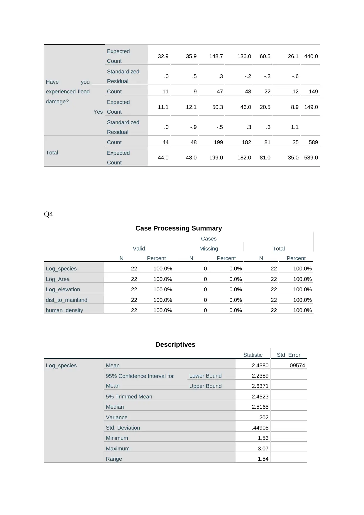
No Count 33 39 152 134 59 23 440
Secure Best Marks with AI Grader
Need help grading? Try our AI Grader for instant feedback on your assignments.
Have you
experienced flood
damage?
Expected
Count 32.9 35.9 148.7 136.0 60.5 26.1 440.0
Standardized
Residual .0 .5 .3 -.2 -.2 -.6
Yes
Count 11 9 47 48 22 12 149
Expected
Count 11.1 12.1 50.3 46.0 20.5 8.9 149.0
Standardized
Residual .0 -.9 -.5 .3 .3 1.1
Total
Count 44 48 199 182 81 35 589
Expected
Count 44.0 48.0 199.0 182.0 81.0 35.0 589.0
Q4
Case Processing Summary
Cases
Valid Missing Total
N Percent N Percent N Percent
Log_species 22 100.0% 0 0.0% 22 100.0%
Log_Area 22 100.0% 0 0.0% 22 100.0%
Log_elevation 22 100.0% 0 0.0% 22 100.0%
dist_to_mainland 22 100.0% 0 0.0% 22 100.0%
human_density 22 100.0% 0 0.0% 22 100.0%
Descriptives
Statistic Std. Error
Log_species Mean 2.4380 .09574
95% Confidence Interval for
Mean
Lower Bound 2.2389
Upper Bound 2.6371
5% Trimmed Mean 2.4523
Median 2.5165
Variance .202
Std. Deviation .44905
Minimum 1.53
Maximum 3.07
Range 1.54
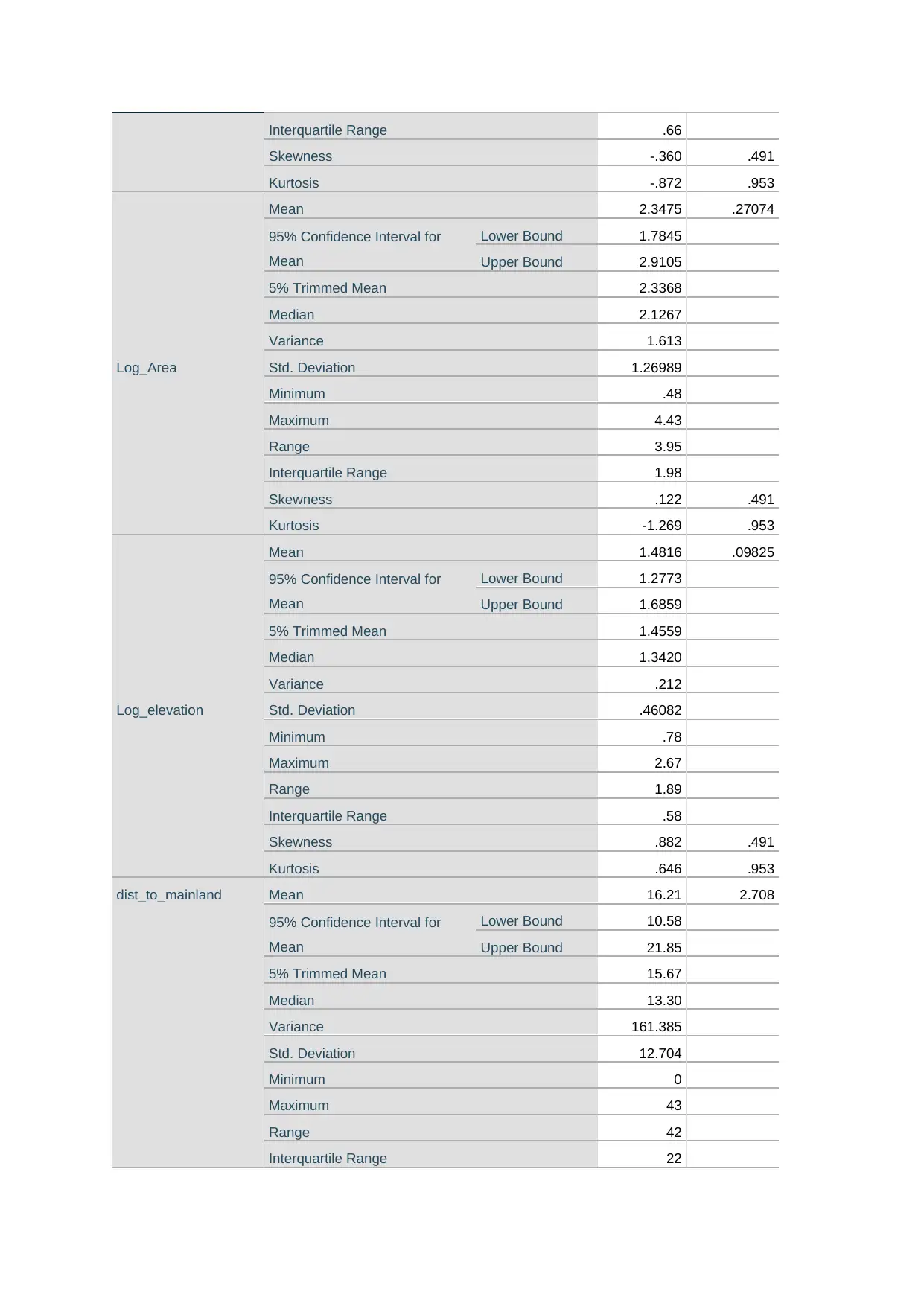
Interquartile Range .66
Skewness -.360 .491
Kurtosis -.872 .953
Log_Area
Mean 2.3475 .27074
95% Confidence Interval for
Mean
Lower Bound 1.7845
Upper Bound 2.9105
5% Trimmed Mean 2.3368
Median 2.1267
Variance 1.613
Std. Deviation 1.26989
Minimum .48
Maximum 4.43
Range 3.95
Interquartile Range 1.98
Skewness .122 .491
Kurtosis -1.269 .953
Log_elevation
Mean 1.4816 .09825
95% Confidence Interval for
Mean
Lower Bound 1.2773
Upper Bound 1.6859
5% Trimmed Mean 1.4559
Median 1.3420
Variance .212
Std. Deviation .46082
Minimum .78
Maximum 2.67
Range 1.89
Interquartile Range .58
Skewness .882 .491
Kurtosis .646 .953
dist_to_mainland Mean 16.21 2.708
95% Confidence Interval for
Mean
Lower Bound 10.58
Upper Bound 21.85
5% Trimmed Mean 15.67
Median 13.30
Variance 161.385
Std. Deviation 12.704
Minimum 0
Maximum 43
Range 42
Interquartile Range 22
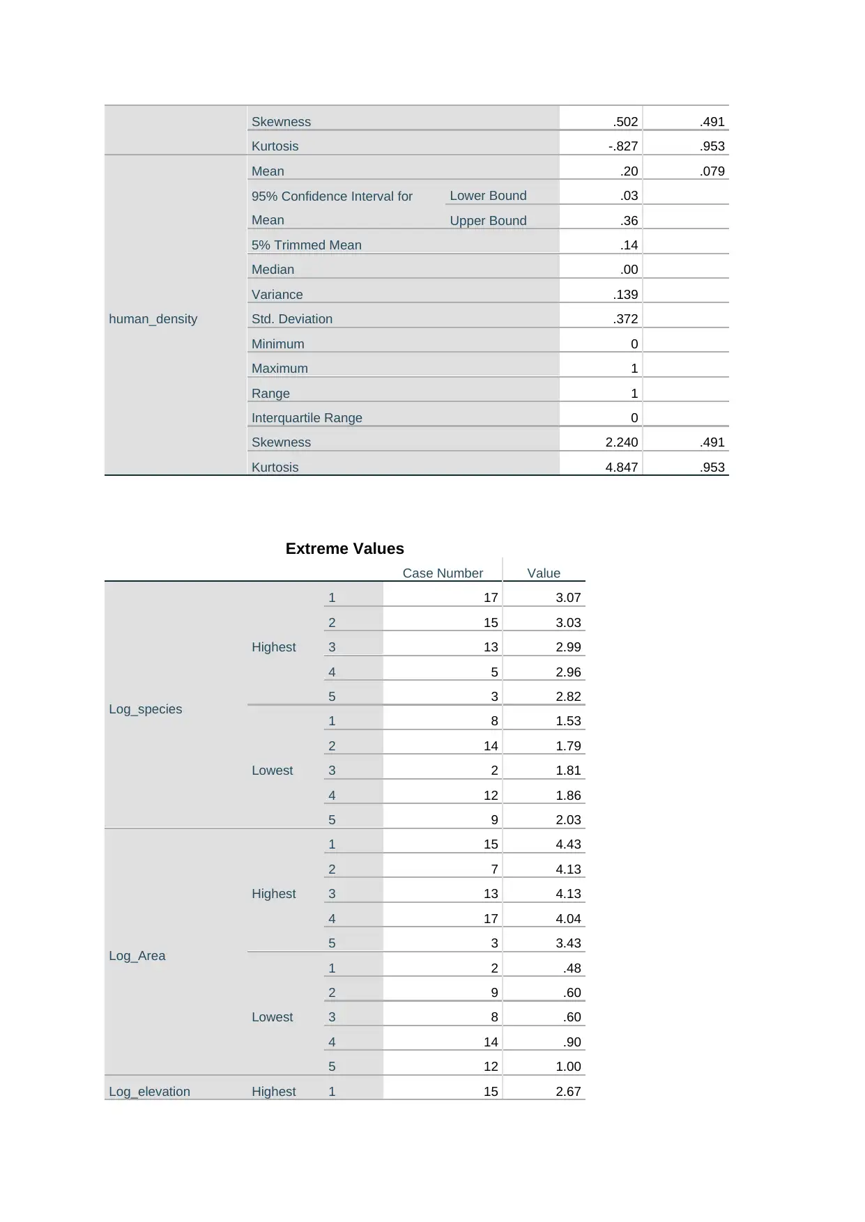
Skewness .502 .491
Kurtosis -.827 .953
human_density
Mean .20 .079
95% Confidence Interval for
Mean
Lower Bound .03
Upper Bound .36
5% Trimmed Mean .14
Median .00
Variance .139
Std. Deviation .372
Minimum 0
Maximum 1
Range 1
Interquartile Range 0
Skewness 2.240 .491
Kurtosis 4.847 .953
Extreme Values
Case Number Value
Log_species
Highest
1 17 3.07
2 15 3.03
3 13 2.99
4 5 2.96
5 3 2.82
Lowest
1 8 1.53
2 14 1.79
3 2 1.81
4 12 1.86
5 9 2.03
Log_Area
Highest
1 15 4.43
2 7 4.13
3 13 4.13
4 17 4.04
5 3 3.43
Lowest
1 2 .48
2 9 .60
3 8 .60
4 14 .90
5 12 1.00
Log_elevation Highest 1 15 2.67
Paraphrase This Document
Need a fresh take? Get an instant paraphrase of this document with our AI Paraphraser
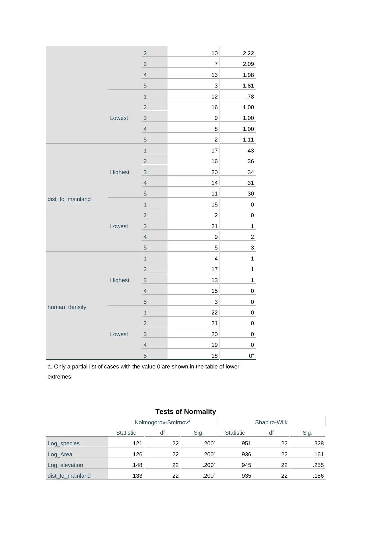
2 10 2.22
3 7 2.09
4 13 1.98
5 3 1.81
Lowest
1 12 .78
2 16 1.00
3 9 1.00
4 8 1.00
5 2 1.11
dist_to_mainland
Highest
1 17 43
2 16 36
3 20 34
4 14 31
5 11 30
Lowest
1 15 0
2 2 0
3 21 1
4 9 2
5 5 3
human_density
Highest
1 4 1
2 17 1
3 13 1
4 15 0
5 3 0
Lowest
1 22 0
2 21 0
3 20 0
4 19 0
5 18 0a
a. Only a partial list of cases with the value 0 are shown in the table of lower
extremes.
Tests of Normality
Kolmogorov-Smirnova Shapiro-Wilk
Statistic df Sig. Statistic df Sig.
Log_species .121 22 .200* .951 22 .328
Log_Area .126 22 .200* .936 22 .161
Log_elevation .148 22 .200* .945 22 .255
dist_to_mainland .133 22 .200* .935 22 .156
human_density .344 22 .000 .612 22 .000
*. This is a lower bound of the true significance.
a. Lilliefors Significance Correction
Regression
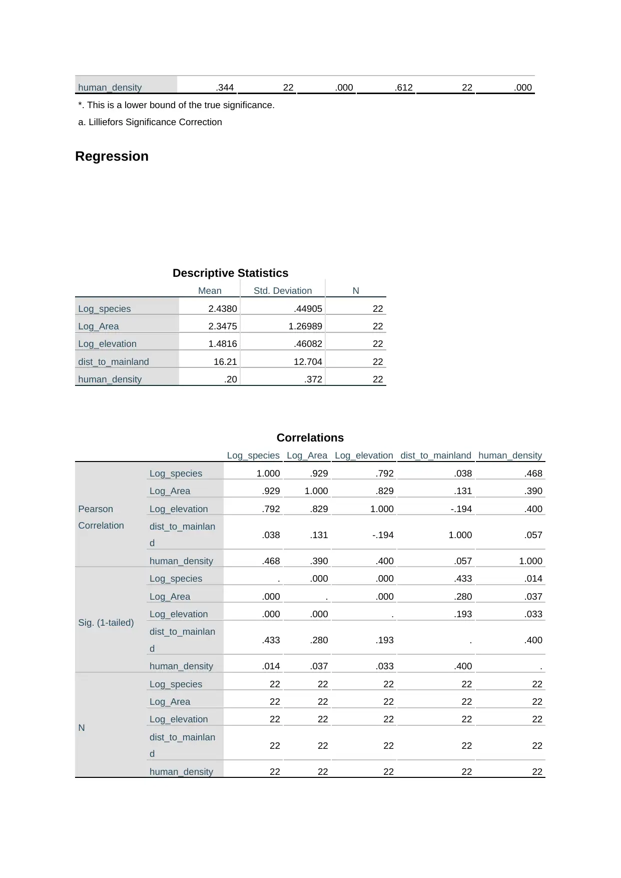
Descriptive Statistics
Mean Std. Deviation N
Log_species 2.4380 .44905 22
Log_Area 2.3475 1.26989 22
Log_elevation 1.4816 .46082 22
dist_to_mainland 16.21 12.704 22
human_density .20 .372 22
Correlations
Log_species Log_Area Log_elevation dist_to_mainland human_density
Pearson
Correlation
Log_species 1.000 .929 .792 .038 .468
Log_Area .929 1.000 .829 .131 .390
Log_elevation .792 .829 1.000 -.194 .400
dist_to_mainlan
d .038 .131 -.194 1.000 .057
human_density .468 .390 .400 .057 1.000
Sig. (1-tailed)
Log_species . .000 .000 .433 .014
Log_Area .000 . .000 .280 .037
Log_elevation .000 .000 . .193 .033
dist_to_mainlan
d .433 .280 .193 . .400
human_density .014 .037 .033 .400 .
N
Log_species 22 22 22 22 22
Log_Area 22 22 22 22 22
Log_elevation 22 22 22 22 22
dist_to_mainlan
d 22 22 22 22 22
human_density 22 22 22 22 22
*. This is a lower bound of the true significance.
a. Lilliefors Significance Correction
Regression
Descriptive Statistics
Mean Std. Deviation N
Log_species 2.4380 .44905 22
Log_Area 2.3475 1.26989 22
Log_elevation 1.4816 .46082 22
dist_to_mainland 16.21 12.704 22
human_density .20 .372 22
Correlations
Log_species Log_Area Log_elevation dist_to_mainland human_density
Pearson
Correlation
Log_species 1.000 .929 .792 .038 .468
Log_Area .929 1.000 .829 .131 .390
Log_elevation .792 .829 1.000 -.194 .400
dist_to_mainlan
d .038 .131 -.194 1.000 .057
human_density .468 .390 .400 .057 1.000
Sig. (1-tailed)
Log_species . .000 .000 .433 .014
Log_Area .000 . .000 .280 .037
Log_elevation .000 .000 . .193 .033
dist_to_mainlan
d .433 .280 .193 . .400
human_density .014 .037 .033 .400 .
N
Log_species 22 22 22 22 22
Log_Area 22 22 22 22 22
Log_elevation 22 22 22 22 22
dist_to_mainlan
d 22 22 22 22 22
human_density 22 22 22 22 22
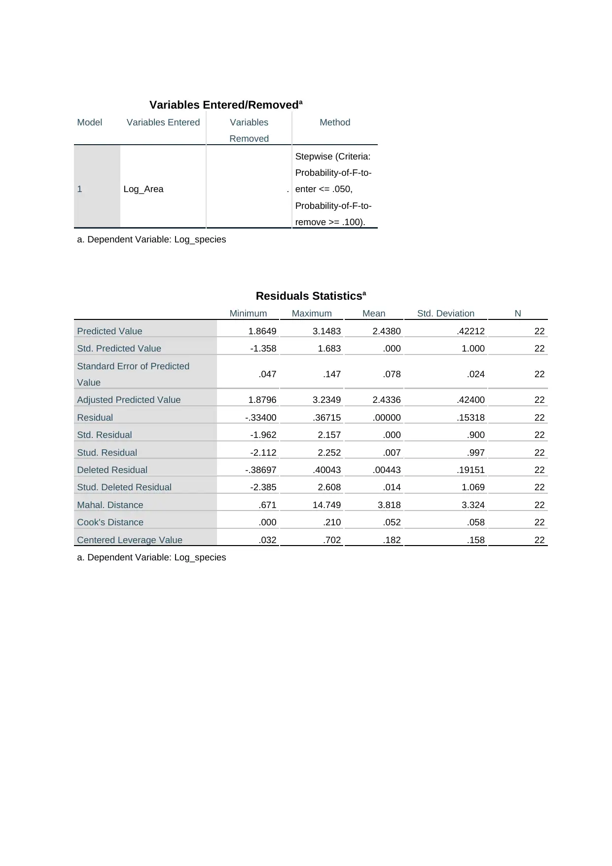
Variables Entered/Removeda
Model Variables Entered Variables
Removed
Method
1 Log_Area .
Stepwise (Criteria:
Probability-of-F-to-
enter <= .050,
Probability-of-F-to-
remove >= .100).
a. Dependent Variable: Log_species
Residuals Statisticsa
Minimum Maximum Mean Std. Deviation N
Predicted Value 1.8649 3.1483 2.4380 .42212 22
Std. Predicted Value -1.358 1.683 .000 1.000 22
Standard Error of Predicted
Value .047 .147 .078 .024 22
Adjusted Predicted Value 1.8796 3.2349 2.4336 .42400 22
Residual -.33400 .36715 .00000 .15318 22
Std. Residual -1.962 2.157 .000 .900 22
Stud. Residual -2.112 2.252 .007 .997 22
Deleted Residual -.38697 .40043 .00443 .19151 22
Stud. Deleted Residual -2.385 2.608 .014 1.069 22
Mahal. Distance .671 14.749 3.818 3.324 22
Cook's Distance .000 .210 .052 .058 22
Centered Leverage Value .032 .702 .182 .158 22
a. Dependent Variable: Log_species
1 out of 52
Related Documents


Your All-in-One AI-Powered Toolkit for Academic Success.
+13062052269
info@desklib.com
Available 24*7 on WhatsApp / Email
![[object Object]](/_next/static/media/star-bottom.7253800d.svg)
Unlock your academic potential
© 2024 | Zucol Services PVT LTD | All rights reserved.