ICT110: Data Analysis Report on Causes of Death in Queensland
VerifiedAdded on 2023/03/31
|13
|2299
|177
Report
AI Summary
This report presents a data analysis of the causes of death in Queensland from 1997 to 2017, aiming to draw significant conclusions for practical applications and further research. The analysis includes K-means cluster analysis, which categorizes years to highlight differences in average death rates due to various factors, and linear regression analysis to demonstrate how the number of deaths changes over time. Data was sourced from the Australian government website and cleaned using Excel 2014, with analysis performed using the R statistical tool. The report covers one-variable and two-variable analyses, examining diseases of the nervous system, mental and behavioral disorders, and their correlation with time. Advanced analysis includes K-means clustering to group years based on death causes and linear regression to model the relationship between specific causes of death (infectious diseases, cancer) and time, revealing statistically significant increasing trends.

Data Analysis report of Causes of Death in Queensland
Name of the Student:
Name of the University:
Author Note:
Name of the Student:
Name of the University:
Author Note:
Paraphrase This Document
Need a fresh take? Get an instant paraphrase of this document with our AI Paraphraser
1
Author Name
Data analysis report of Causes of death in queensland
Table of Contents
Introduction...............................................................................................................................2
Data setup..................................................................................................................................2
Explanatory Data Analysis..........................................................................................................2
One Variable Analysis.............................................................................................................2
Two Variable Analysis............................................................................................................4
Advanced Analysis......................................................................................................................5
K-means Cluster Analysis.......................................................................................................5
Linear regression Analysis......................................................................................................7
Conclusion................................................................................................................................11
Reflections................................................................................................................................11
Reference and Bibliography.....................................................................................................12
2
Author Name
Data analysis report of Causes of death in queensland
Introduction
This report presents the analysis of deaths due to various reasons from 1997 to 2017
in Queensland. The report tries to draw significant conclusions that can be useful for
practical life and further studies. The paper deals with a k means cluster analysis which
makes sub groups of year to present significant differences among average death rates due
to several reasons. The linear regressions shows how the number of death is changing over
the year. The data is collected from the Australian government website to analyse the
reasons of death in Queensland. The data cleaning is completed in Excel 2014 and the
analysis is done with help of open source statistical tool pack R.
Data setup
The data was not prepared for the analysis so some changes were made using excel.
In this stage the name of the variables are edited, the transpose of the data set is taken for
the analysis to describe the variables across year. After all these steps the excel file was
imported in R for the further analysis. The following codes were used accordingly.
ucdq<- readxl::read_xlsx(file.choose()) # import and read the excel file in R
The following codes are to upload the library which were used for the analysis.
library(RColorBrewer)
library(ggplot2)
library(stats4)
library(cluster)
Now, to omit the missing variables na.omit function is used some them are
mentioned below and thus the data is prepared for the further analysis (Little and Rubin
2019).
na.omit(ucdq$`Cause of death`)
na.omit(ucdq$`Certain infectious and parasitic diseases`)
na.omit(ucdq$`Neoplasms (cancer)`)
na.omit(ucdq$`Trachea, bronchus and lung`)
na.omit(ucdq$`Melanoma of skin`)
na.omit(ucdq$Breast)
Explanatory Data Analysis
One Variable Analysis
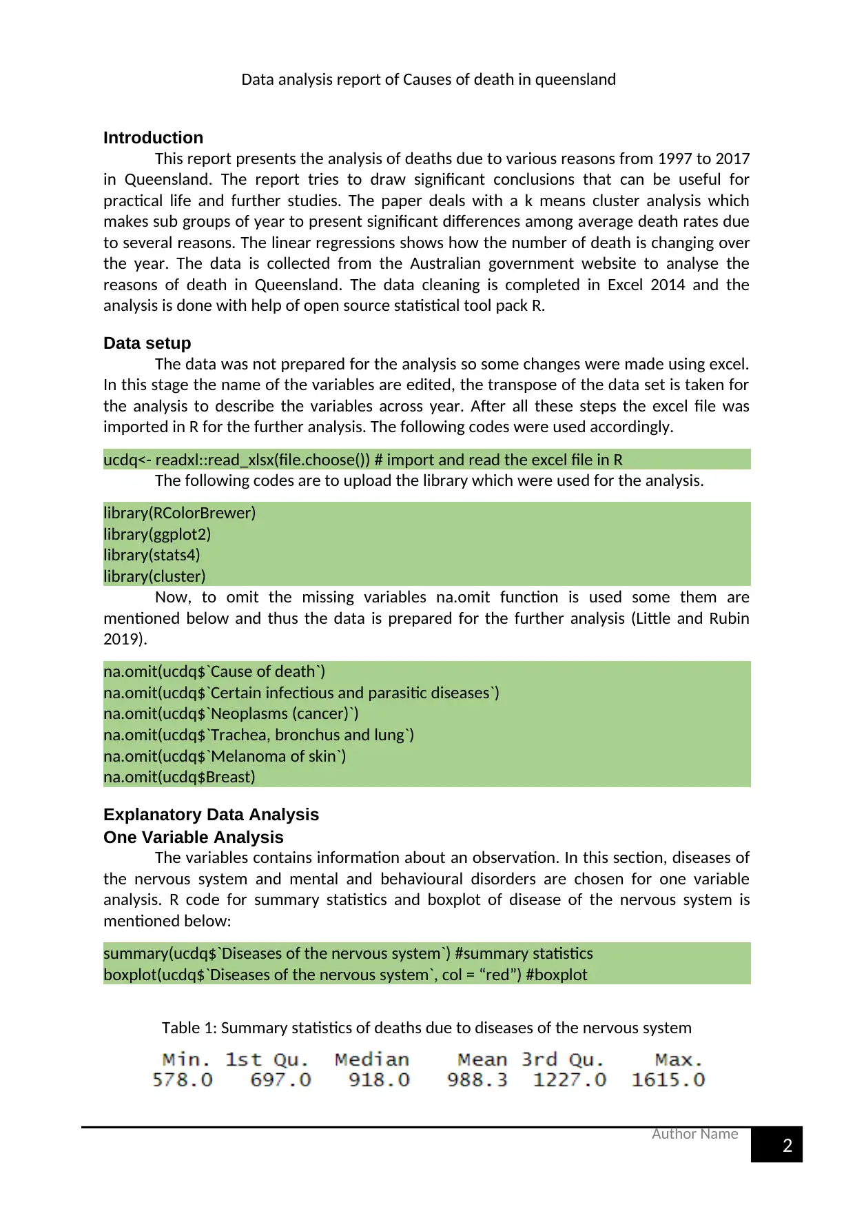
The variables contains information about an observation. In this section, diseases of
the nervous system and mental and behavioural disorders are chosen for one variable
analysis. R code for summary statistics and boxplot of disease of the nervous system is
mentioned below:
summary(ucdq$`Diseases of the nervous system`) #summary statistics
boxplot(ucdq$`Diseases of the nervous system`, col = “red”) #boxplot
Table 1: Summary statistics of deaths due to diseases of the nervous system
Author Name
Data analysis report of Causes of death in queensland
Introduction
This report presents the analysis of deaths due to various reasons from 1997 to 2017
in Queensland. The report tries to draw significant conclusions that can be useful for
practical life and further studies. The paper deals with a k means cluster analysis which
makes sub groups of year to present significant differences among average death rates due
to several reasons. The linear regressions shows how the number of death is changing over
the year. The data is collected from the Australian government website to analyse the
reasons of death in Queensland. The data cleaning is completed in Excel 2014 and the
analysis is done with help of open source statistical tool pack R.
Data setup
The data was not prepared for the analysis so some changes were made using excel.
In this stage the name of the variables are edited, the transpose of the data set is taken for
the analysis to describe the variables across year. After all these steps the excel file was
imported in R for the further analysis. The following codes were used accordingly.
ucdq<- readxl::read_xlsx(file.choose()) # import and read the excel file in R
The following codes are to upload the library which were used for the analysis.
library(RColorBrewer)
library(ggplot2)
library(stats4)
library(cluster)
Now, to omit the missing variables na.omit function is used some them are
mentioned below and thus the data is prepared for the further analysis (Little and Rubin
2019).
na.omit(ucdq$`Cause of death`)
na.omit(ucdq$`Certain infectious and parasitic diseases`)
na.omit(ucdq$`Neoplasms (cancer)`)
na.omit(ucdq$`Trachea, bronchus and lung`)
na.omit(ucdq$`Melanoma of skin`)
na.omit(ucdq$Breast)
Explanatory Data Analysis
One Variable Analysis
The variables contains information about an observation. In this section, diseases of
the nervous system and mental and behavioural disorders are chosen for one variable
analysis. R code for summary statistics and boxplot of disease of the nervous system is
mentioned below:
summary(ucdq$`Diseases of the nervous system`) #summary statistics
boxplot(ucdq$`Diseases of the nervous system`, col = “red”) #boxplot
Table 1: Summary statistics of deaths due to diseases of the nervous system
⊘ This is a preview!⊘
Do you want full access?
Subscribe today to unlock all pages.
Trusted by 1+ million students worldwide
3
Author Name
Data analysis report of Causes of death in queensland
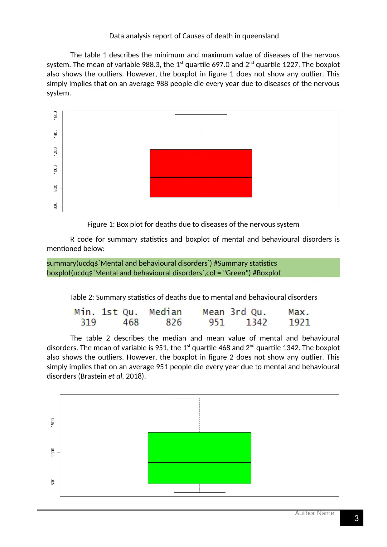
The table 1 describes the minimum and maximum value of diseases of the nervous
system. The mean of variable 988.3, the 1st quartile 697.0 and 2nd quartile 1227. The boxplot
also shows the outliers. However, the boxplot in figure 1 does not show any outlier. This
simply implies that on an average 988 people die every year due to diseases of the nervous
system.
Figure 1: Box plot for deaths due to diseases of the nervous system
R code for summary statistics and boxplot of mental and behavioural disorders is
mentioned below:
summary(ucdq$`Mental and behavioural disorders`) #Summary statistics
boxplot(ucdq$`Mental and behavioural disorders`,col = "Green") #Boxplot
Table 2: Summary statistics of deaths due to mental and behavioural disorders
The table 2 describes the median and mean value of mental and behavioural
disorders. The mean of variable is 951, the 1st quartile 468 and 2nd quartile 1342. The boxplot
also shows the outliers. However, the boxplot in figure 2 does not show any outlier. This
simply implies that on an average 951 people die every year due to mental and behavioural
disorders (Brastein et al. 2018).
Author Name
Data analysis report of Causes of death in queensland
The table 1 describes the minimum and maximum value of diseases of the nervous
system. The mean of variable 988.3, the 1st quartile 697.0 and 2nd quartile 1227. The boxplot
also shows the outliers. However, the boxplot in figure 1 does not show any outlier. This
simply implies that on an average 988 people die every year due to diseases of the nervous
system.
Figure 1: Box plot for deaths due to diseases of the nervous system
R code for summary statistics and boxplot of mental and behavioural disorders is
mentioned below:
summary(ucdq$`Mental and behavioural disorders`) #Summary statistics
boxplot(ucdq$`Mental and behavioural disorders`,col = "Green") #Boxplot
Table 2: Summary statistics of deaths due to mental and behavioural disorders
The table 2 describes the median and mean value of mental and behavioural
disorders. The mean of variable is 951, the 1st quartile 468 and 2nd quartile 1342. The boxplot
also shows the outliers. However, the boxplot in figure 2 does not show any outlier. This
simply implies that on an average 951 people die every year due to mental and behavioural
disorders (Brastein et al. 2018).
Paraphrase This Document
Need a fresh take? Get an instant paraphrase of this document with our AI Paraphraser
4
Author Name
Data analysis report of Causes of death in queensland
Figure 2: Box plot for deaths due to mental and behavioural disorders
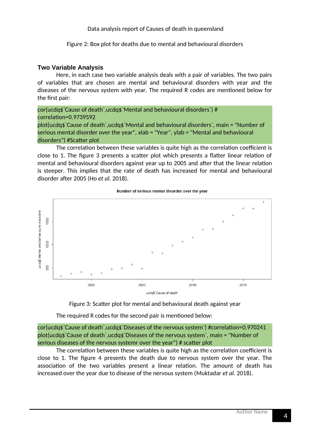
Two Variable Analysis
Here, in each case two variable analysis deals with a pair of variables. The two pairs
of variables that are chosen are mental and behavioural disorders with year and the
diseases of the nervous system with year. The required R codes are mentioned below for
the first pair:
cor(ucdq$`Cause of death`,ucdq$`Mental and behavioural disorders`) #
correlation=0.9739592
plot(ucdq$`Cause of death`,ucdq$`Mental and behavioural disorders`, main = "Number of
serious mental disorder over the year", xlab = "Year", ylab = "Mental and behavioural
disorders") #Scatter plot
The correlation between these variables is quite high as the correlation coefficient is
close to 1. The figure 3 presents a scatter plot which presents a flatter linear relation of
mental and behavioural disorders against year up to 2005 and after that the linear relation
is steeper. This implies that the rate of death has increased for mental and behavioural
disorder after 2005 (Ho et al. 2018).
Figure 3: Scatter plot for mental and behavioural death against year
The required R codes for the second pair is mentioned below:
cor(ucdq$`Cause of death`,ucdq$`Diseases of the nervous system`) #correlation=0.970241
plot(ucdq$`Cause of death`,ucdq$`Diseases of the nervous system`, main = "Number of
serious diseases of the nervous systemr over the year") # scatter plot
The correlation between these variables is quite high as the correlation coefficient is
close to 1. The figure 4 presents the death due to nervous system over the year. The
association of the two variables present a linear relation. The amount of death has
increased over the year due to disease of the nervous system (Muktadar et al. 2018).
Author Name
Data analysis report of Causes of death in queensland
Figure 2: Box plot for deaths due to mental and behavioural disorders
Two Variable Analysis
Here, in each case two variable analysis deals with a pair of variables. The two pairs
of variables that are chosen are mental and behavioural disorders with year and the
diseases of the nervous system with year. The required R codes are mentioned below for
the first pair:
cor(ucdq$`Cause of death`,ucdq$`Mental and behavioural disorders`) #
correlation=0.9739592
plot(ucdq$`Cause of death`,ucdq$`Mental and behavioural disorders`, main = "Number of
serious mental disorder over the year", xlab = "Year", ylab = "Mental and behavioural
disorders") #Scatter plot
The correlation between these variables is quite high as the correlation coefficient is
close to 1. The figure 3 presents a scatter plot which presents a flatter linear relation of
mental and behavioural disorders against year up to 2005 and after that the linear relation
is steeper. This implies that the rate of death has increased for mental and behavioural
disorder after 2005 (Ho et al. 2018).
Figure 3: Scatter plot for mental and behavioural death against year
The required R codes for the second pair is mentioned below:
cor(ucdq$`Cause of death`,ucdq$`Diseases of the nervous system`) #correlation=0.970241
plot(ucdq$`Cause of death`,ucdq$`Diseases of the nervous system`, main = "Number of
serious diseases of the nervous systemr over the year") # scatter plot
The correlation between these variables is quite high as the correlation coefficient is
close to 1. The figure 4 presents the death due to nervous system over the year. The
association of the two variables present a linear relation. The amount of death has
increased over the year due to disease of the nervous system (Muktadar et al. 2018).
5
Author Name
Data analysis report of Causes of death in queensland
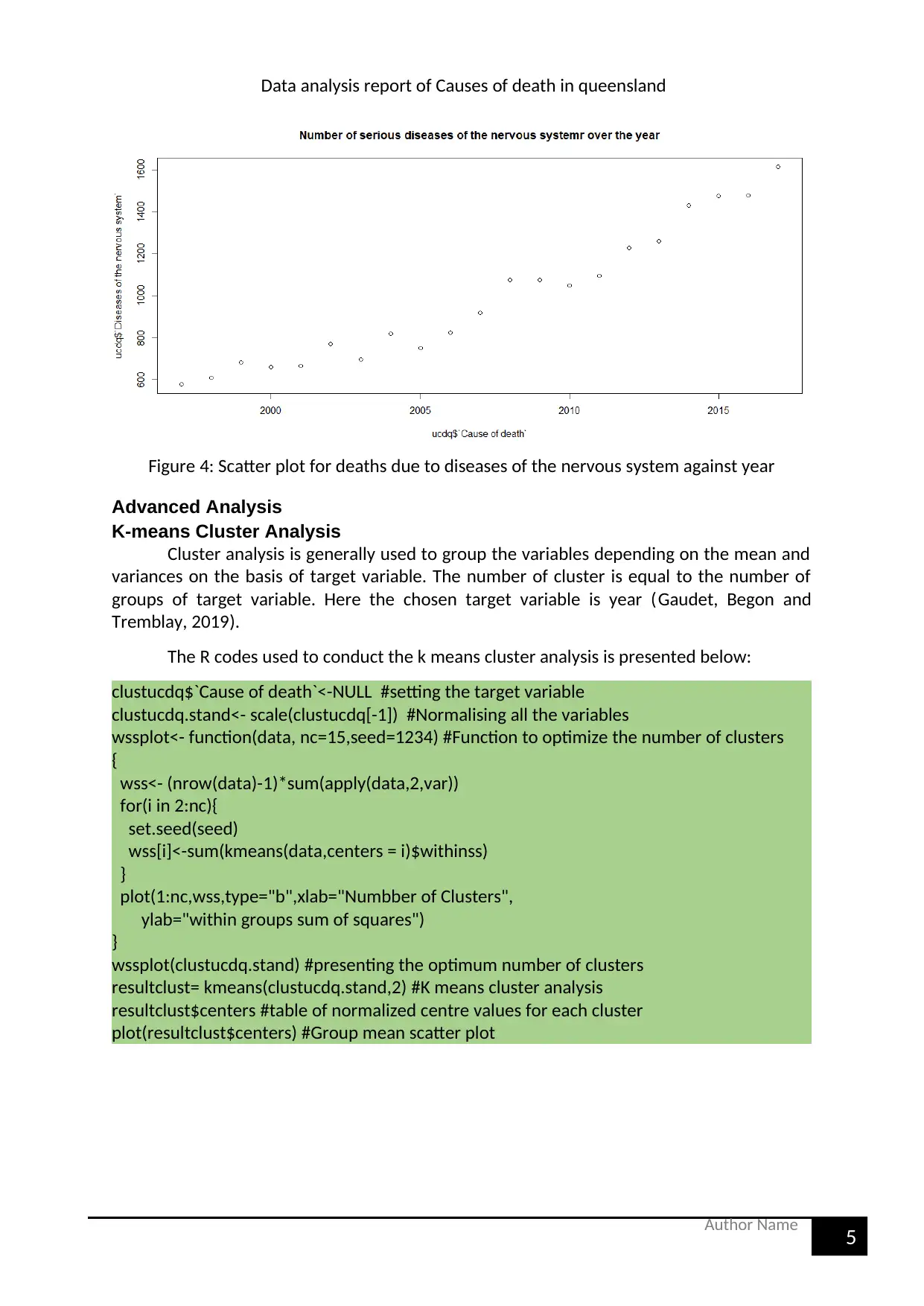
Figure 4: Scatter plot for deaths due to diseases of the nervous system against year
Advanced Analysis
K-means Cluster Analysis
Cluster analysis is generally used to group the variables depending on the mean and
variances on the basis of target variable. The number of cluster is equal to the number of
groups of target variable. Here the chosen target variable is year (Gaudet, Begon and
Tremblay, 2019).
The R codes used to conduct the k means cluster analysis is presented below:
clustucdq$`Cause of death`<-NULL #setting the target variable
clustucdq.stand<- scale(clustucdq[-1]) #Normalising all the variables
wssplot<- function(data, nc=15,seed=1234) #Function to optimize the number of clusters
{
wss<- (nrow(data)-1)*sum(apply(data,2,var))
for(i in 2:nc){
set.seed(seed)
wss[i]<-sum(kmeans(data,centers = i)$withinss)
}
plot(1:nc,wss,type="b",xlab="Numbber of Clusters",
ylab="within groups sum of squares")
}
wssplot(clustucdq.stand) #presenting the optimum number of clusters
resultclust= kmeans(clustucdq.stand,2) #K means cluster analysis
resultclust$centers #table of normalized centre values for each cluster
plot(resultclust$centers) #Group mean scatter plot
Author Name
Data analysis report of Causes of death in queensland
Figure 4: Scatter plot for deaths due to diseases of the nervous system against year
Advanced Analysis
K-means Cluster Analysis
Cluster analysis is generally used to group the variables depending on the mean and
variances on the basis of target variable. The number of cluster is equal to the number of
groups of target variable. Here the chosen target variable is year (Gaudet, Begon and
Tremblay, 2019).
The R codes used to conduct the k means cluster analysis is presented below:
clustucdq$`Cause of death`<-NULL #setting the target variable
clustucdq.stand<- scale(clustucdq[-1]) #Normalising all the variables
wssplot<- function(data, nc=15,seed=1234) #Function to optimize the number of clusters
{
wss<- (nrow(data)-1)*sum(apply(data,2,var))
for(i in 2:nc){
set.seed(seed)
wss[i]<-sum(kmeans(data,centers = i)$withinss)
}
plot(1:nc,wss,type="b",xlab="Numbber of Clusters",
ylab="within groups sum of squares")
}
wssplot(clustucdq.stand) #presenting the optimum number of clusters
resultclust= kmeans(clustucdq.stand,2) #K means cluster analysis
resultclust$centers #table of normalized centre values for each cluster
plot(resultclust$centers) #Group mean scatter plot
⊘ This is a preview!⊘
Do you want full access?
Subscribe today to unlock all pages.
Trusted by 1+ million students worldwide
6
Author Name
Data analysis report of Causes of death in queensland
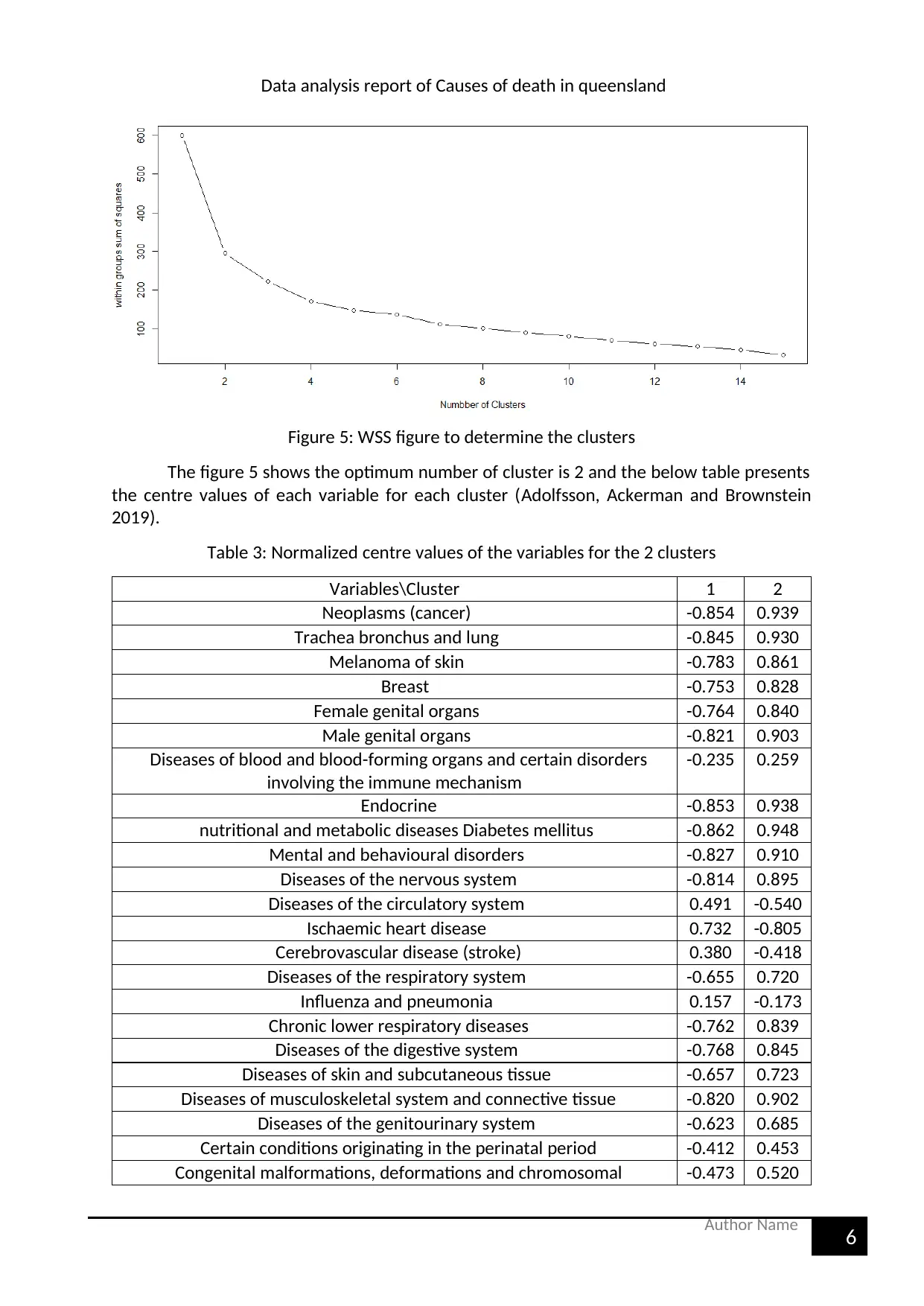
Figure 5: WSS figure to determine the clusters
The figure 5 shows the optimum number of cluster is 2 and the below table presents
the centre values of each variable for each cluster (Adolfsson, Ackerman and Brownstein
2019).
Table 3: Normalized centre values of the variables for the 2 clusters
Variables\Cluster 1 2
Neoplasms (cancer) -0.854 0.939
Trachea bronchus and lung -0.845 0.930
Melanoma of skin -0.783 0.861
Breast -0.753 0.828
Female genital organs -0.764 0.840
Male genital organs -0.821 0.903
Diseases of blood and blood-forming organs and certain disorders
involving the immune mechanism
-0.235 0.259
Endocrine -0.853 0.938
nutritional and metabolic diseases Diabetes mellitus -0.862 0.948
Mental and behavioural disorders -0.827 0.910
Diseases of the nervous system -0.814 0.895
Diseases of the circulatory system 0.491 -0.540
Ischaemic heart disease 0.732 -0.805
Cerebrovascular disease (stroke) 0.380 -0.418
Diseases of the respiratory system -0.655 0.720
Influenza and pneumonia 0.157 -0.173
Chronic lower respiratory diseases -0.762 0.839
Diseases of the digestive system -0.768 0.845
Diseases of skin and subcutaneous tissue -0.657 0.723
Diseases of musculoskeletal system and connective tissue -0.820 0.902
Diseases of the genitourinary system -0.623 0.685
Certain conditions originating in the perinatal period -0.412 0.453
Congenital malformations, deformations and chromosomal -0.473 0.520
Author Name
Data analysis report of Causes of death in queensland
Figure 5: WSS figure to determine the clusters
The figure 5 shows the optimum number of cluster is 2 and the below table presents
the centre values of each variable for each cluster (Adolfsson, Ackerman and Brownstein
2019).
Table 3: Normalized centre values of the variables for the 2 clusters
Variables\Cluster 1 2
Neoplasms (cancer) -0.854 0.939
Trachea bronchus and lung -0.845 0.930
Melanoma of skin -0.783 0.861
Breast -0.753 0.828
Female genital organs -0.764 0.840
Male genital organs -0.821 0.903
Diseases of blood and blood-forming organs and certain disorders
involving the immune mechanism
-0.235 0.259
Endocrine -0.853 0.938
nutritional and metabolic diseases Diabetes mellitus -0.862 0.948
Mental and behavioural disorders -0.827 0.910
Diseases of the nervous system -0.814 0.895
Diseases of the circulatory system 0.491 -0.540
Ischaemic heart disease 0.732 -0.805
Cerebrovascular disease (stroke) 0.380 -0.418
Diseases of the respiratory system -0.655 0.720
Influenza and pneumonia 0.157 -0.173
Chronic lower respiratory diseases -0.762 0.839
Diseases of the digestive system -0.768 0.845
Diseases of skin and subcutaneous tissue -0.657 0.723
Diseases of musculoskeletal system and connective tissue -0.820 0.902
Diseases of the genitourinary system -0.623 0.685
Certain conditions originating in the perinatal period -0.412 0.453
Congenital malformations, deformations and chromosomal -0.473 0.520
Paraphrase This Document
Need a fresh take? Get an instant paraphrase of this document with our AI Paraphraser
7
Author Name
Data analysis report of Causes of death in queensland
abnormalities
Symptoms, signs and abnormal clinical and laboratory findings, not
elsewhere classified
-0.198 0.218
External causes of morbidity and mortality -0.810 0.891
Transport accidents 0.422 -0.465
Falls -0.790 0.869
Accidental drowning and submersion 0.001 -0.001
Intentional self-harm (suicide) -0.682 0.750
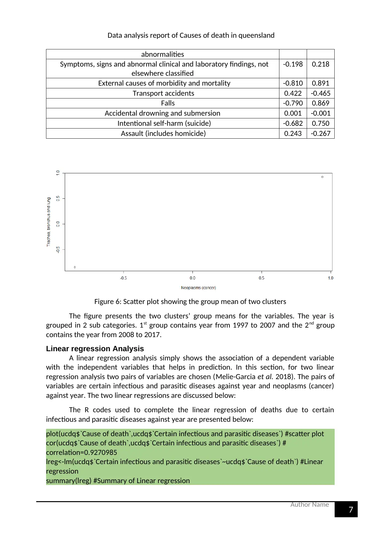
Assault (includes homicide) 0.243 -0.267
Figure 6: Scatter plot showing the group mean of two clusters
The figure presents the two clusters’ group means for the variables. The year is
grouped in 2 sub categories. 1st group contains year from 1997 to 2007 and the 2nd group
contains the year from 2008 to 2017.
Linear regression Analysis
A linear regression analysis simply shows the association of a dependent variable
with the independent variables that helps in prediction. In this section, for two linear
regression analysis two pairs of variables are chosen (Melie-Garcia et al. 2018). The pairs of
variables are certain infectious and parasitic diseases against year and neoplasms (cancer)
against year. The two linear regressions are discussed below:
The R codes used to complete the linear regression of deaths due to certain
infectious and parasitic diseases against year are presented below:
plot(ucdq$`Cause of death`,ucdq$`Certain infectious and parasitic diseases`) #scatter plot
cor(ucdq$`Cause of death`,ucdq$`Certain infectious and parasitic diseases`) #
correlation=0.9270985
lreg<-lm(ucdq$`Certain infectious and parasitic diseases`~ucdq$`Cause of death`) #Linear
regression
summary(lreg) #Summary of Linear regression
Author Name
Data analysis report of Causes of death in queensland
abnormalities
Symptoms, signs and abnormal clinical and laboratory findings, not
elsewhere classified
-0.198 0.218
External causes of morbidity and mortality -0.810 0.891
Transport accidents 0.422 -0.465
Falls -0.790 0.869
Accidental drowning and submersion 0.001 -0.001
Intentional self-harm (suicide) -0.682 0.750
Assault (includes homicide) 0.243 -0.267
Figure 6: Scatter plot showing the group mean of two clusters
The figure presents the two clusters’ group means for the variables. The year is
grouped in 2 sub categories. 1st group contains year from 1997 to 2007 and the 2nd group
contains the year from 2008 to 2017.
Linear regression Analysis
A linear regression analysis simply shows the association of a dependent variable
with the independent variables that helps in prediction. In this section, for two linear
regression analysis two pairs of variables are chosen (Melie-Garcia et al. 2018). The pairs of
variables are certain infectious and parasitic diseases against year and neoplasms (cancer)
against year. The two linear regressions are discussed below:
The R codes used to complete the linear regression of deaths due to certain
infectious and parasitic diseases against year are presented below:
plot(ucdq$`Cause of death`,ucdq$`Certain infectious and parasitic diseases`) #scatter plot
cor(ucdq$`Cause of death`,ucdq$`Certain infectious and parasitic diseases`) #
correlation=0.9270985
lreg<-lm(ucdq$`Certain infectious and parasitic diseases`~ucdq$`Cause of death`) #Linear
regression
summary(lreg) #Summary of Linear regression
8
Author Name
Data analysis report of Causes of death in queensland
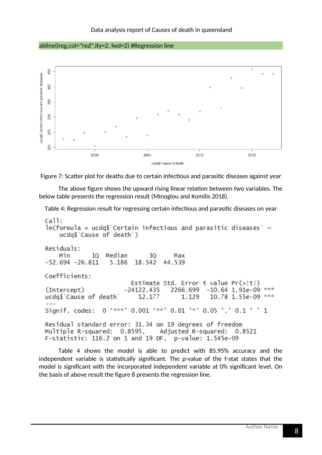
abline(lreg,col="red",lty=2, lwd=2) #Regression line
Figure 7: Scatter plot for deaths due to certain infectious and parasitic diseases against year
The above figure shows the upward rising linear relation between two variables. The
below table presents the regression result (Minoglou and Komilis 2018).
Table 4: Regression result for regressing certain infectious and parasitic diseases on year
Table 4 shows the model is able to predict with 85.95% accuracy and the
independent variable is statistically significant. The p-value of the f-stat states that the
model is significant with the incorporated independent variable at 0% significant level. On
the basis of above result the figure 8 presents the regression line.
Author Name
Data analysis report of Causes of death in queensland
abline(lreg,col="red",lty=2, lwd=2) #Regression line
Figure 7: Scatter plot for deaths due to certain infectious and parasitic diseases against year
The above figure shows the upward rising linear relation between two variables. The
below table presents the regression result (Minoglou and Komilis 2018).
Table 4: Regression result for regressing certain infectious and parasitic diseases on year
Table 4 shows the model is able to predict with 85.95% accuracy and the
independent variable is statistically significant. The p-value of the f-stat states that the
model is significant with the incorporated independent variable at 0% significant level. On
the basis of above result the figure 8 presents the regression line.
⊘ This is a preview!⊘
Do you want full access?
Subscribe today to unlock all pages.
Trusted by 1+ million students worldwide
9
Author Name
Data analysis report of Causes of death in queensland
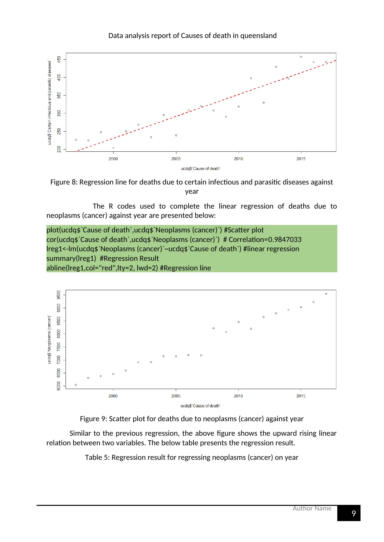
Figure 8: Regression line for deaths due to certain infectious and parasitic diseases against
year
The R codes used to complete the linear regression of deaths due to
neoplasms (cancer) against year are presented below:
plot(ucdq$`Cause of death`,ucdq$`Neoplasms (cancer)`) #Scatter plot
cor(ucdq$`Cause of death`,ucdq$`Neoplasms (cancer)`) # Correlation=0.9847033
lreg1<-lm(ucdq$`Neoplasms (cancer)`~ucdq$`Cause of death`) #linear regression
summary(lreg1) #Regression Result
abline(lreg1,col="red",lty=2, lwd=2) #Regression line
Figure 9: Scatter plot for deaths due to neoplasms (cancer) against year
Similar to the previous regression, the above figure shows the upward rising linear
relation between two variables. The below table presents the regression result.
Table 5: Regression result for regressing neoplasms (cancer) on year
Author Name
Data analysis report of Causes of death in queensland
Figure 8: Regression line for deaths due to certain infectious and parasitic diseases against
year
The R codes used to complete the linear regression of deaths due to
neoplasms (cancer) against year are presented below:
plot(ucdq$`Cause of death`,ucdq$`Neoplasms (cancer)`) #Scatter plot
cor(ucdq$`Cause of death`,ucdq$`Neoplasms (cancer)`) # Correlation=0.9847033
lreg1<-lm(ucdq$`Neoplasms (cancer)`~ucdq$`Cause of death`) #linear regression
summary(lreg1) #Regression Result
abline(lreg1,col="red",lty=2, lwd=2) #Regression line
Figure 9: Scatter plot for deaths due to neoplasms (cancer) against year
Similar to the previous regression, the above figure shows the upward rising linear
relation between two variables. The below table presents the regression result.
Table 5: Regression result for regressing neoplasms (cancer) on year
Paraphrase This Document
Need a fresh take? Get an instant paraphrase of this document with our AI Paraphraser
10
Author Name
Data analysis report of Causes of death in queensland
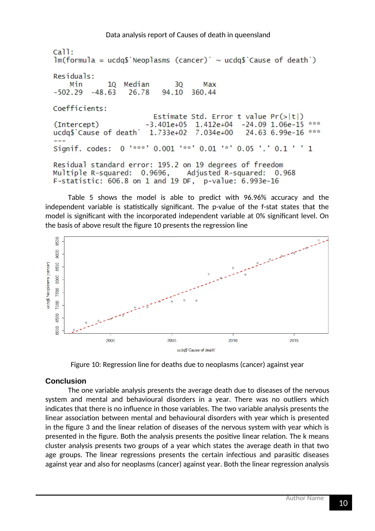
Table 5 shows the model is able to predict with 96.96% accuracy and the
independent variable is statistically significant. The p-value of the f-stat states that the
model is significant with the incorporated independent variable at 0% significant level. On
the basis of above result the figure 10 presents the regression line
Figure 10: Regression line for deaths due to neoplasms (cancer) against year
Conclusion
The one variable analysis presents the average death due to diseases of the nervous
system and mental and behavioural disorders in a year. There was no outliers which
indicates that there is no influence in those variables. The two variable analysis presents the
linear association between mental and behavioural disorders with year which is presented
in the figure 3 and the linear relation of diseases of the nervous system with year which is
presented in the figure. Both the analysis presents the positive linear relation. The k means
cluster analysis presents two groups of a year which states the average death in that two
age groups. The linear regressions presents the certain infectious and parasitic diseases
against year and also for neoplasms (cancer) against year. Both the linear regression analysis
Author Name
Data analysis report of Causes of death in queensland
Table 5 shows the model is able to predict with 96.96% accuracy and the
independent variable is statistically significant. The p-value of the f-stat states that the
model is significant with the incorporated independent variable at 0% significant level. On
the basis of above result the figure 10 presents the regression line
Figure 10: Regression line for deaths due to neoplasms (cancer) against year
Conclusion
The one variable analysis presents the average death due to diseases of the nervous
system and mental and behavioural disorders in a year. There was no outliers which
indicates that there is no influence in those variables. The two variable analysis presents the
linear association between mental and behavioural disorders with year which is presented
in the figure 3 and the linear relation of diseases of the nervous system with year which is
presented in the figure. Both the analysis presents the positive linear relation. The k means
cluster analysis presents two groups of a year which states the average death in that two
age groups. The linear regressions presents the certain infectious and parasitic diseases
against year and also for neoplasms (cancer) against year. Both the linear regression analysis
11
Author Name
Data analysis report of Causes of death in queensland
says the relationship is statistically significant at % significance level. This means over the
year average death due to both the reasons incorporated in the analysis is increasing.
Reflections
There are a huge number of techniques to analyse the qualitative and quantitative
variable. The set of data used in the analysis is a time series data where time series analysis
can be done to predict the future disease for which the number of deaths will be higher and
the lower. This can help the scientists to do research on that disease to control its effects by
providing a plenty of time.
⊘ This is a preview!⊘
Do you want full access?
Subscribe today to unlock all pages.
Trusted by 1+ million students worldwide
1 out of 13
Related Documents


Your All-in-One AI-Powered Toolkit for Academic Success.
+13062052269
info@desklib.com
Available 24*7 on WhatsApp / Email
![[object Object]](/_next/static/media/star-bottom.7253800d.svg)
Unlock your academic potential
Copyright © 2020–2025 A2Z Services. All Rights Reserved. Developed and managed by ZUCOL.