Data Mining Techniques: Decision Tree, Naive Bayes, and K-Nearest Neighbor Algorithms

This article discusses the different data mining techniques such as decision tree, naive bayes, and k-nearest neighbor algorithms. It explains the basic assumptions when creating decision trees and the concept of confusion matrix in summarizing the performance of classification algorithms. The article also provides insights on the difference in performance between the algorithms.

Data mining.
Name.
Institutional affiliation.

Calcification can be performed either in a structured or unstructured way. For this part of the
analysis, we used classification which is the techniques where we do a recognition of a given
case of algorithms. Classification aims at identifying the new data and how this new data will fall
into the research objectives This classification will look at three major factors that can be used to
identify the data mining techniques
Decision Tree
The main aim of the decision tree is actually to create a model that can be used in predicting the
class or even the value by learning the rules and data management. Understanding decision tree
algorism is not very hard but it comparison is somehow complicated. A decision tree is where
each and every node represents its feature. From the analysis, each link while each outcomes. In
This analysis the main thing is to create a decision tree that is similar to the entire process.
Understanding decision tree is very easy when it is compared with the classification algorithms.
It tries to solve every problem using a tree replacement representation (Ting, 2017). Each and
every internal nodes corresponds to an attribute and each and every leaf will correspond to a
class label. When using a decision to predict the label for a god record, the process starts with the
roots of the tree. We do a comparison of the root t attribute. Based on this comparison, we must
follows the corresponding to that value and jumps to the next value. The record comparison
continues using an internal record tree until the entire process reach the leaf node. Knowing how
the modelled decision can work, in predicting the target class or the value now the understating
of how to create decision tree model is brought forward.

Basic assumption when creating decision tree.
When we create decision tree, we assume that the entire process considered a roots.
Features values are actually preferred to be categorical. In case the values continues then they are
considered to be discrete and building model for the entire tree.
The record used are distributed recursively based on the attributes of the entire value. The order
of placing the attribute in the internal node by using same statistical approach. Research shows
that decision tree follows the concept of sum of product representation. The images formed on
weka shows how the values can be compatible. This description is also known as a descriptive or
disjunction or normal form. For every class, every root of the tree pose the same class
Naive Bayes
To demonstrate this concept, we must consider an example displays in an illustration based on
procedure and experimental factors. Based on the indication, the objective is either a green or the
intakes is to put a classification based on the data that arrived first. It also define which level the
decision tree is at the time of analysis. When two variables appear such as twice green, then we
conclude that there is a reasonable membership and case study. The baiyan analysis recognize
this as prior profitability. Prior profitability are actually based on the previous experience. In this
case we have a better number of information compared to the actually data and the number of
repeated happenings.
To get the exact information according to the data required, we must formulate a probability.
After doing this, we must perform a classification. This is done easily because the objects are

well clustered. This makes it known that there are more data and object vicinity compared to the
new cases that belonged to the color. To have a real measure of likelihood we must draw a circle
around X which is a combination of numbers and irrespective of their own classes and labels.
After this, we have to do a detailed calculated.
Although we have an assumption that the independent and dependent variable are not always
very accurate, this process does simplify the dramatically since the class conditions and densities
are calculated separately for every variable. Byuyan performs a reduction of density estimation
and task to a one dimetnila kernel density estimations. Moreover, this assumption does not
necessarily give a different probability of certain boundaries.
K-nearest neighbor algorithms.
This is anon parametric method that I used t clarify and perform a regression analysis. In both
cases, the input considered the k-the closet training in the feature space. In simple terms, the
structure of this is basically determent and it is proving very useful in the real world. This is not
basically meant to obey te assumptions produced by some of the other algorithms. In this regard,
this algorithms can be one of the choices used when there is a serious distribution of data. This
algorithms is also called lazy algorithms because according to the analysis, it side not use the
training data and does not point to many particular generalization. There is not explicit training
or if there is any it is very minimal. The output seen in this case is a class based membership
which means that is can be predicted. In this algorithm, the objects is basically classified a
majority of votes complied with the neighbors and is assigned to class of the most common
among the group. It is also used to regression. In most cases, the output is value of the object in
question and due to this, the average value is received from the K nearest neighbor.

Part 2.
A confusion matrix is defined as a techniques used in summarizing the performance of the
classification algorithms. When we consider the accuracy of the data presented without looking
at the factor observed, we might get a misleading results because other resources may not be
considered. Presenting a confusion matrix has given us a better idea of what the classification
model is and we have given a right data as it is marking. When data is more than 2 classes the
accuracy according to the observation is 80%. We are not sure whether this value is true because
it is predicted and it may not give the model of the entire learning. When data lacks even number
as this particular data, accuracy may be achieve at 90% level however this is not considered as a
good level either because it belongs to one class that always predicting the most common class
values.
Confusion matrix in this case has been used to predict the results of the problems. The project
summarizes the number of correct and incorrect predictors with the count values and Brocken
values and they are taken back to each and every class (Ohsaki & Ralescu et al., 2017). This is
the main idea of the confusion matrix. The confession matrix also has shown how the
classification model is confused when main predictions. It also gives a clear insight which is not
only based on the errors committed by the classifier but is more importantly the type of error
which is currently being made.
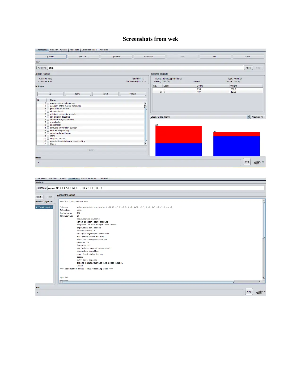
The weka machine displays a confusion matrix automatically when the estimations are done.
This modeling is done on weka explorer interface. In weka, the confusion matric is listed at the
bottom and the entire presentation is also presented. For the confusion matrix, different letter are
assigned to ascertain the predicted values. In most cases, the problem of prediction models is to

have a good performance making a prediction which is based on a new data. This makes it very
important to use a more reliable techniques to help evaluate the models that is to be evaluated.
The observation provides a suggestion that the more reliable the estimation is, the more
performance and the further one can go on with the estimation. This also dictates how confident
the operational will be.
Is there a difference in performance between the algorithms?
From the observation, there is a difference in the performance in the algorithms. The difference
is evidence when using the K-nearest neighbor which presents a suggestion that the nearest
neighbor will be selected. This is proves to give a more accurate information in comparison to
the rest of the algorithms (Deng & Mahadevan, 2016). While the main aim of a decision tree is to
solve every problem using a tree replacement representation. Each and every internal nodes
corresponds to an attribute and each and every leaf will correspond to a class label. When using a
decision to predict the label for a god record, the process starts with the roots of the tree. We do a
comparison of the root t attribute, the K nearest neighbor will be more concentrative on the issue
of the nearest tree.

Screenshots from wek

References
Ting, K. M. (2017). Confusion matrix. In Encyclopedia of Machine Learning and Data Mining
(pp. 260-260). Springer, Boston, MA.
Ohsaki, M., Wang, P., Matsuda, K., Katagiri, S., Watanabe, H., & Ralescu, A. (2017).
Confusion-matrix-based kernel logistic regression for imbalanced data classification. IEEE
Transactions on Knowledge and Data Engineering, 29(9), 1806-1819.
Deng, X., Liu, Q., Deng, Y., & Mahadevan, S. (2016). An improved method to construct basic
probability assignment based on the confusion matrix for classification problem. Information
Sciences, 340, 250-261.
Tsirigos, K. D., Peters, C., Shu, N., Käll, L., & Elofsson, A. (2015). The TOPCONS web server
for consensus prediction of membrane protein topology and signal peptides. Nucleic acids
research, 43(W1), W401-W407.