Data Modeling in R: Simulation, Probability, and MLE Analysis

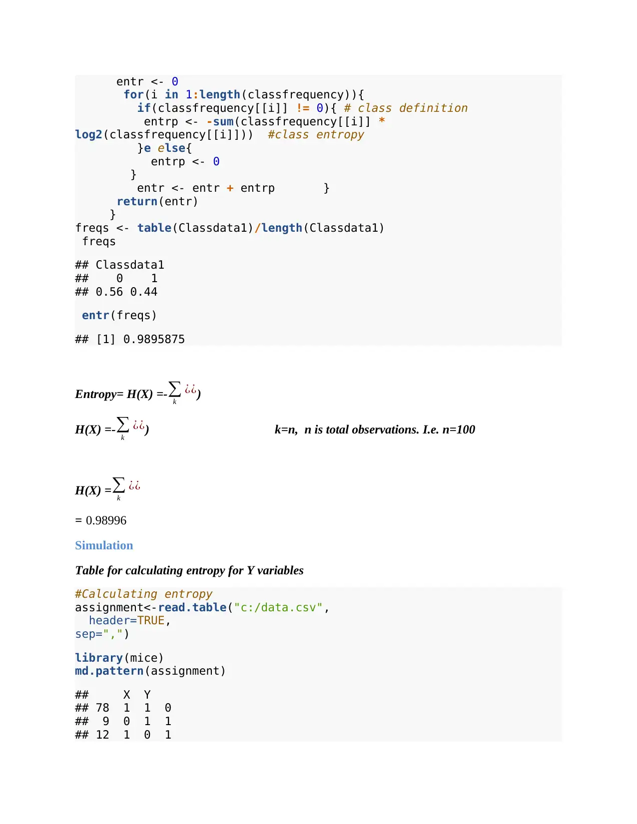
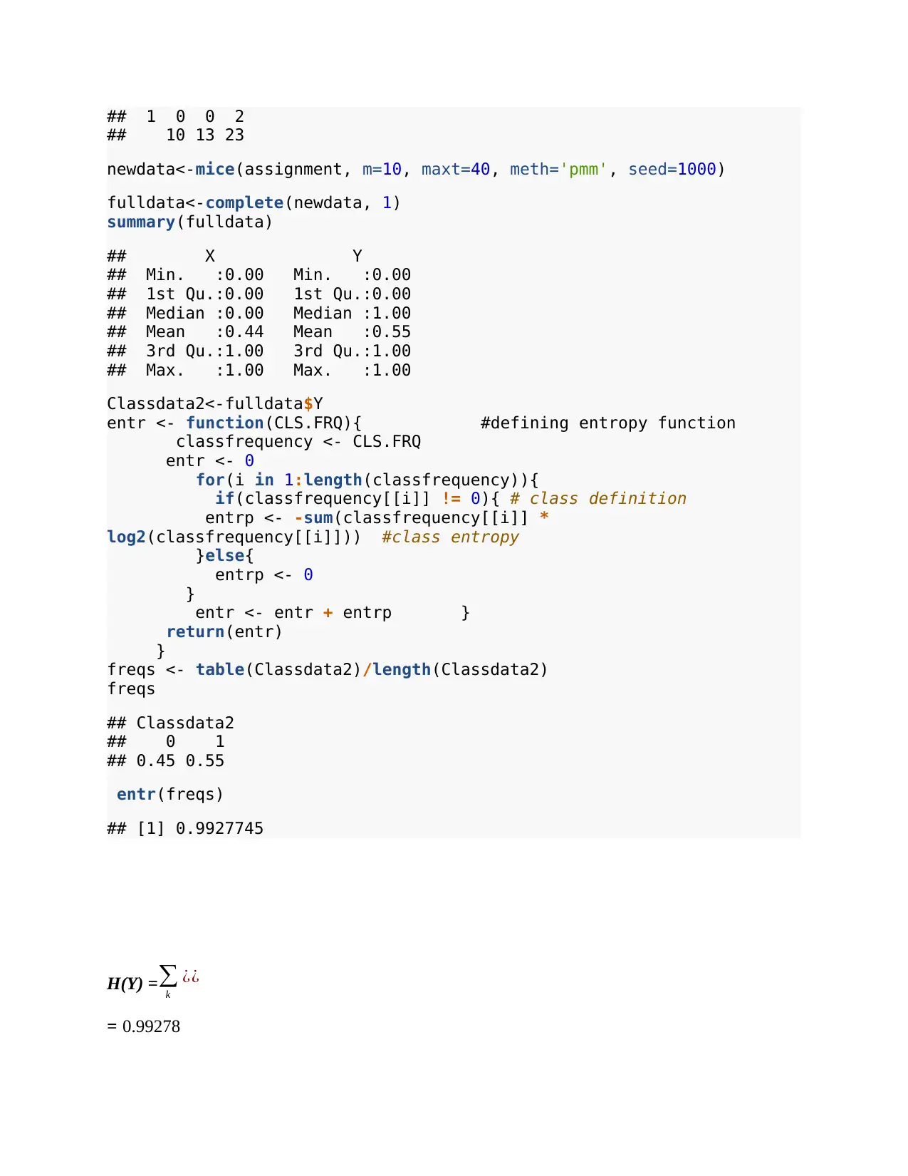
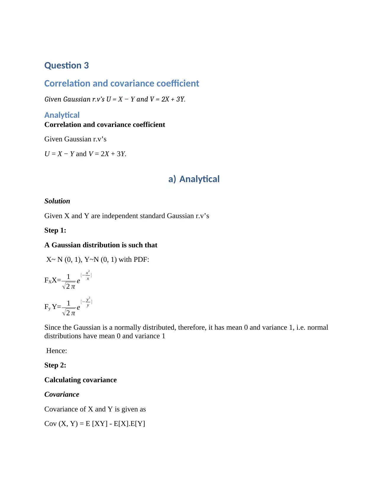
This assignment focuses on data modeling using R, addressing key concepts such as conditional probability, entropy, correlation, maximum likelihood estimation (MLE), and the central limit theorem. The conditional probability question involves calculating the probability of specific events when tossing a fair die, solved both analytically and through simulation. The entropy section deals with handling missing data in a Boolean dataset, calculating probability distributions, and determining entropy for X and Y variables. Correlation and covariance coefficients are explored using Gaussian random variables, with both analytical solutions and simulations. The MLE section focuses on determining the maximum likelihood estimator from a Poisson distribution. Finally, the assignment justifies the central limit theorem using different sample sizes and R code for a normal Poisson distribution. The solutions are supported by R code and detailed explanations.

Data_Modelling
Student:
March 31, 2018
Title: Data modeling in R
Assignment type: Analytical computation and
simulation, in R
Student Name: XXX
Tutor’s Name: XXX
Due date: XX-XX

Question 1
Conditional probability
A dice is tossed 7 times: A being probability of each value appearing at least once, B probability
outcome is alternate numbers, hence:
Analytical
Conditional prob(probability) Of A given B is-
PR(A|B)
Such that
Pr(a and b) = PR(A|B)*P(B)
Where, Pr(a and b) is the joint probability of A and B.
Therefore:
PR(A|B) = P (A∧B)
P(B)
Probability of a number on a dice occurring at least once i.e. event A
k =7 (n=sample number)
p=0.167 (p=probability of event occurring)
q=0.833 (q=probability of event not occurring)
Hence given a binomial probability b(x; k, P) = { k !
[ X ! ( k −X ) !]} × PX× (1- p k-X)
( [ 7 !
6 !1 !∗0.1676∗0.8331
] )
6
=0.000126
Probability of a number occurring but not adjacent, i.e. without replacement, event B
Given the probability a number occurs is 0.000126 then the probability that the succeeding
number is not the same is such that the succeeding number is either odd followed by even or
even followed by odd, hence
Probability of even= 7 !
6 !1!∗0.1676∗0.8331=0.000126

And
Probability of odd= 7 !
6 !1!∗0.1676∗0.8331=0.000126
However given that joint the probability of A(odd) and B(even) is given by P(A ∩B)
In such that P(A) + P(B)
But P(A)=0.000126, P(A)=0.000126
Therefore
0.000126 + 0.000126=0.000252
Alternatively
0.000126×2 =0.000252
Hence:
pr(b)=0.000252
Therefore calculating conditional probability:
PR(A|B) = P (A∧B)
P(B)
But
Pr(a and b) = Pr (a) * Pr (b) = 0.000126∗0.000252=0.000000031
Hence:
Pr ( a/ b ) = Pr ( a∧b )
P ( b ) = 0.000000031
0.000252 =0.000126
Pr (a/b) = 0.000126
Simulation
#calculating probability of event occurring when rolling dice once,
i.e. p
dicex<-6
n<-1
dice.prob<-function(dices) prod(1/dices)
dice.prob(c(n,dicex))
## [1] 0.1666667

#calculating probability of an event not occurring when rolling a
dice, i.e. q
dicex<-6
n<-1
dice.prob<-function(dices) 1-prod(1/dices)
dice.prob(c(n,dicex))
## [1] 0.8333333
#calculating probability of a number occurring at least once in 7 dice
tosses, i.e. event A
eventA<-dbinom(6, size=7, prob=0.1666667)
eventA
## [1] 0.0001250287
#calculating probability of event B
evendice<-(dbinom(6, size=7, prob=0.1666667))
odddice<-(dbinom(6, size=7, prob=0.1666667))
EventB<-evendice+odddice
EventB
## [1] 0.0002500574
#calculating conditional probability for event A given event B p (A/B)
conditprob<-(EventB*eventA)/EventB
conditprob
## [1] 0.0001250287
Question 2
Entropy
Imputing missing data (handling NAs)
#raw data
#imputed data
#summary of imputed and raw data
#histogram of Y variables
assignment<-read.table("c:/data.csv",
header=TRUE,
sep=",")
assignment
newdata<-mice(assignment, m=10, maxt=40, meth='pmm', seed=1000)
fulldata<-complete(newdata, 1)
fulldata
summary(fulldata)

## X Y
## Min. :0.00 Min. :0.00
## 1st Qu.:0.00 1st Qu.:0.00
## Median :0.00 Median :1.00
## Mean :0.44 Mean :0.55
## 3rd Qu.:1.00 3rd Qu.:1.00
## Max. :1.00 Max. :1.00
Classdata1<-fulldata$X
hist(Classdata1)
Classdata1<-fulldata$X
hist(Classdata1)
hist(Classdata1, main="Histogram of class assignment data for x
variables", xlab="X variables", border="blue", col="skyblue",
xlim=c(0,1),las=1,breaks=5)
#raw data
#imputed data
#summary of imputed and raw data
#histogram of Y variables
assignment<-read.table("c:/data.csv",
header=TRUE,
sep=",")
assignment

library(mice)
md.pattern(assignment)
## X Y
## 78 1 1 0
## 9 0 1 1
## 12 1 0 1
## 1 0 0 2
## 10 13 23
newdata<-mice(assignment, m=10, maxt=40, meth='pmm', seed=1000)
fulldata<-complete(newdata, 1)
fulldata
summary(fulldata)
## X Y
## Min. :0.00 Min. :0.00
## 1st Qu.:0.00 1st Qu.:0.00
## Median :0.00 Median :1.00
## Mean :0.44 Mean :0.55
## 3rd Qu.:1.00 3rd Qu.:1.00
## Max. :1.00 Max. :1.00
Classdata2<-fulldata$Y
hist(Classdata2)
Classdata2<-fulldata$Y
hist(Classdata2)
hist(Classdata2, main="Histogram of class assignment data for y
variables", xlab="Y variables", border="blue", col="skyblue",
xlim=c(0,1),las=1,breaks=5)

i Probability.
#calculating probability distributions for X and Y
prop.table(table(fulldata))
## Y
## X 0 1
## 0 0.24 0.32
## 1 0.21 0.23
X Y 0 1 pi 0 0.23 0.32 0.55 1 0.24 0.21 0.45 pj 0.47 0.53 1.00
X
Y
0 1 pi
0 0.23 0.32 0.55
1 0.24 0.21 0.45
pj 0.47 0.53 1.00
Hence from the table:
P(x) =0.47
P(y) =0.55

P(x/y) = P ( x∧Y )
P(Y ) = 0.23
0.55 = 0.41811
P(y/x) = P ( Xand Y )
P( X ) = 0.23
0.47 =0.48936
P(xy)=0.2585
i Entropy
Simulation
Table for calculating entropy for X variables
#raw data
#imputed data
#Calculating entropy
assignment<-read.table("c:/data.csv",
header=TRUE,
sep=",")
library(mice)
## Loading required package: lattice
md.pattern(assignment)
## X Y
## 78 1 1 0
## 9 0 1 1
## 12 1 0 1
## 1 0 0 2
## 10 13 23
newdata<-mice(assignment, m=10, maxt=40, meth='pmm', seed=1000)
fulldata<-complete(newdata, 1)
summary(fulldata)
## X Y
## Min. :0.00 Min. :0.00
## 1st Qu.:0.00 1st Qu.:0.00
## Median :0.00 Median :1.00
## Mean :0.44 Mean :0.55
## 3rd Qu.:1.00 3rd Qu.:1.00
## Max. :1.00 Max. :1.00
Classdata1<-fulldata$X
entr <- function(CLS.FRQ){
classfrequency <- CLS.FRQ

entr <- 0
for(i in 1:length(classfrequency)){
if(classfrequency[[i]] != 0){ # class definition
entrp <- -sum(classfrequency[[i]] *
log2(classfrequency[[i]])) #class entropy
}e else{
entrp <- 0
}
entr <- entr + entrp }
return(entr)
}
freqs <- table(Classdata1)/length(Classdata1)
freqs
## Classdata1
## 0 1
## 0.56 0.44
entr(freqs)
## [1] 0.9895875
Entropy= H(X) =-∑
k
¿¿)
H(X) =-∑
k
¿¿) k=n, n is total observations. I.e. n=100
H(X) =∑
k
¿¿
= 0.98996
Simulation
Table for calculating entropy for Y variables
#Calculating entropy
assignment<-read.table("c:/data.csv",
header=TRUE,
sep=",")
library(mice)
md.pattern(assignment)
## X Y
## 78 1 1 0
## 9 0 1 1
## 12 1 0 1

## 1 0 0 2
## 10 13 23
newdata<-mice(assignment, m=10, maxt=40, meth='pmm', seed=1000)
fulldata<-complete(newdata, 1)
summary(fulldata)
## X Y
## Min. :0.00 Min. :0.00
## 1st Qu.:0.00 1st Qu.:0.00
## Median :0.00 Median :1.00
## Mean :0.44 Mean :0.55
## 3rd Qu.:1.00 3rd Qu.:1.00
## Max. :1.00 Max. :1.00
Classdata2<-fulldata$Y
entr <- function(CLS.FRQ){ #defining entropy function
classfrequency <- CLS.FRQ
entr <- 0
for(i in 1:length(classfrequency)){
if(classfrequency[[i]] != 0){ # class definition
entrp <- -sum(classfrequency[[i]] *
log2(classfrequency[[i]])) #class entropy
}else{
entrp <- 0
}
entr <- entr + entrp }
return(entr)
}
freqs <- table(Classdata2)/length(Classdata2)
freqs
## Classdata2
## 0 1
## 0.45 0.55
entr(freqs)
## [1] 0.9927745
H(Y) =∑
k
¿¿
= 0.99278

H(X|Y )=∑
k
¿¿
= 0.96204
H(Y|X )=∑
k
¿¿
= 0.99962

Question 3
Correlation and covariance coefficient
Given Gaussian r.v’s U = X − Y and V = 2X + 3Y.
Analytical
Correlation and covariance coefficient
Given Gaussian r.v’s
U = X − Y and V = 2X + 3Y.
a) Analytical
Solution
Given X and Y are independent standard Gaussian r.v’s
Step 1:
A Gaussian distribution is such that
X~ N (0, 1), Y~N (0, 1) with PDF:
FXX= 1
√ 2 π e{− x2
x }
Fy Y= 1
√ 2 π e{− y2
y }
Since the Gaussian is a normally distributed, therefore, it has mean 0 and variance 1, i.e. normal
distributions have mean 0 and variance 1
Hence:
Step 2:
Calculating covariance
Covariance
Covariance of X and Y is given as
Cov (X, Y) = E [XY] - E[X].E[Y]