Data Structure and Algorithms - Desklib Online Library

This document discusses the use of algorithms to solve problems, including dynamic programming and greedy algorithms. It also covers data structures and their systematic way of storing data. The document includes examples of binary search trees, the maximum flow problem, and the traveling salesman problem. The motivation for using binary trees is also discussed. The document concludes with references to external sources.

DATA STRUCTURE AND ALGORITHMS
NAME :
REGISTRATION NUMBER :
UNIT CODE :
DATE OF SUBMISSION :

Introduction
Algorithms are set of rules that are used to solve different kind of problems. There are different
types of algorithms that can be applied on different problems and solve them e.g dynamic
programming and greedy algorithms. On the other hand data structure is a systematic way of
storing data for future use. The following shows and describe how some algorithms are used to
problems.

1.
a)
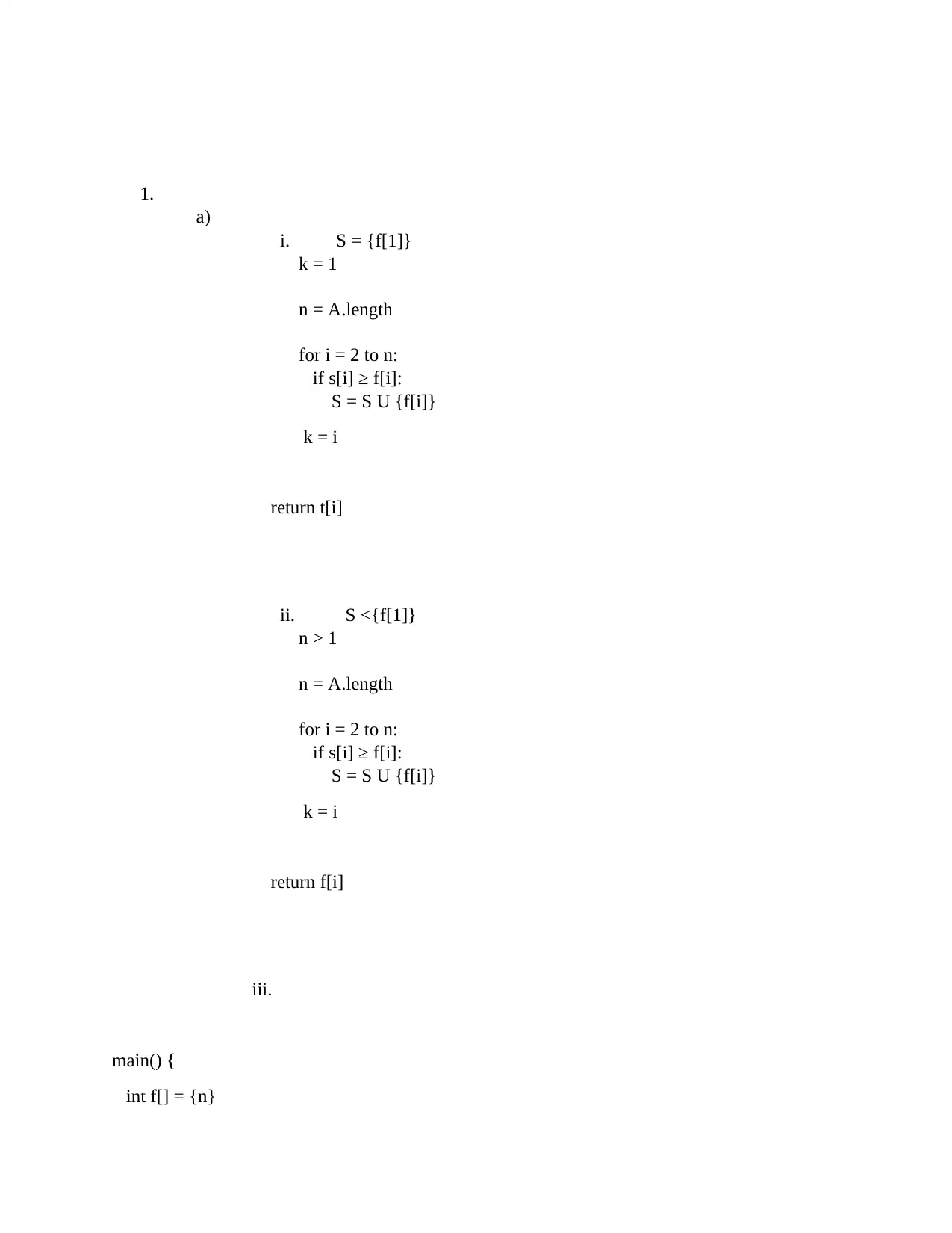
i. S = {f[1]}
k = 1
n = A.length
for i = 2 to n:
if s[i] ≥ f[i]:
S = S U {f[i]}
k = i
return t[i]
ii. S <{f[1]}
n > 1
n = A.length
for i = 2 to n:
if s[i] ≥ f[i]:
S = S U {f[i]}
k = i
return f[i]
iii.
main() {
int f[] = {n}

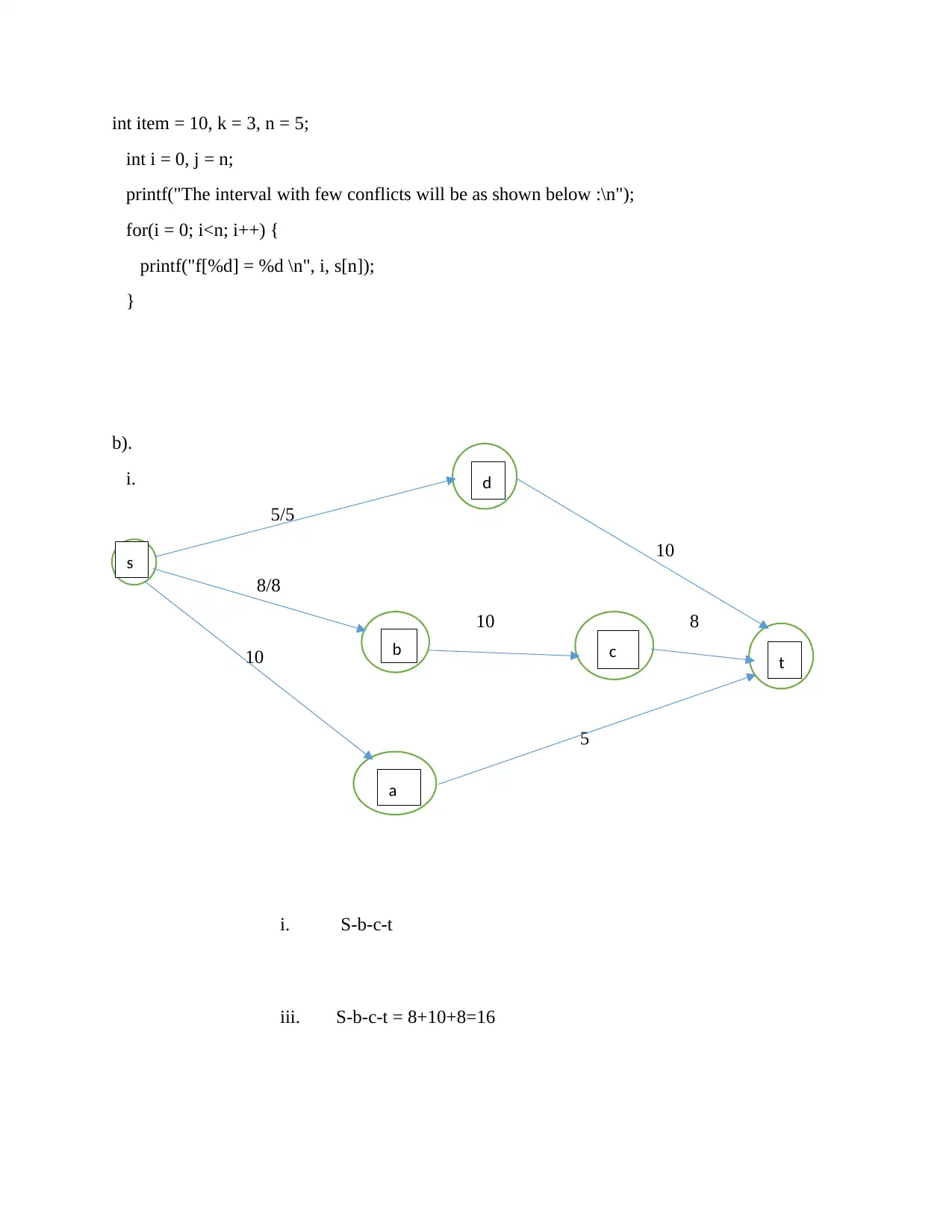
int item = 10, k = 3, n = 5;
int i = 0, j = n;
printf("The interval with few conflicts will be as shown below :\n");
for(i = 0; i<n; i++) {
printf("f[%d] = %d \n", i, s[n]);
}
b).
i.
5/5
10
8/8
10 8
10
5
i. S-b-c-t
iii. S-b-c-t = 8+10+8=16
s
d
a
b c t

c). Maximum flow problem– is a flow that normal involves finding feasible
flows over solo sources (Berg,2008).
Given a graph G= (j∪s, E) where we are to find the largest set of jobs to be
scheduled
N = J∪S∪{J,S}, E' ), is constructed to find the values where by maximum value
of the two will be equal.

2.
a.
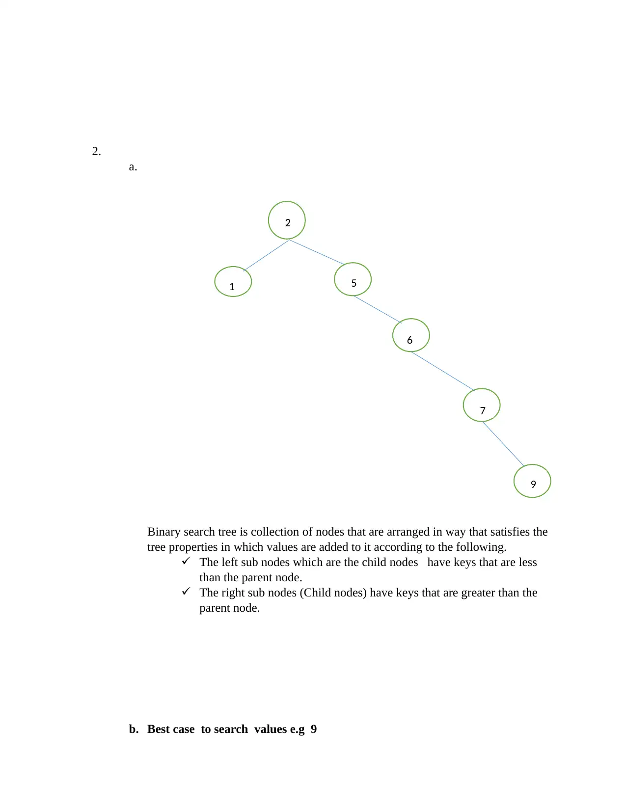
Binary search tree is collection of nodes that are arranged in way that satisfies the
tree properties in which values are added to it according to the following.
 The left sub nodes which are the child nodes have keys that are less
than the parent node.
 The right sub nodes (Child nodes) have keys that are greater than the
parent node.
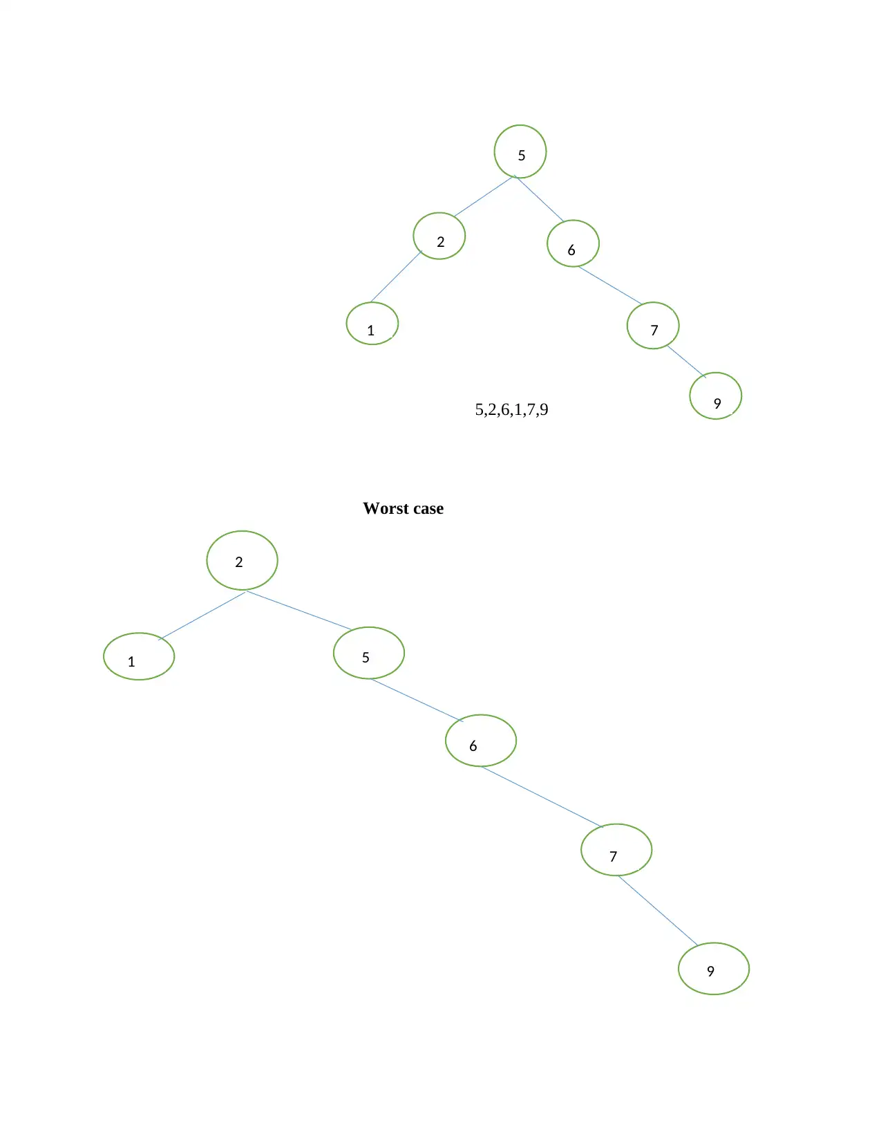
b. Best case to search values e.g 9
2
5
6
7
9
1

5,2,6,1,7,9
Worst case
5
2 6
1 7
9
2
5
6
7
9
1

c.
d. The motivation for using the binary trees according to (Oostenveld,2011).
 Binary trees allow us to accomplish in algorithmic time rather than linear
time.
 They carry out large inserts and deletes in data structures without resorting
them.
 It is very easy to implement lock free data structure from binary tree than
any other type.
 They have high speed and are more efficient.
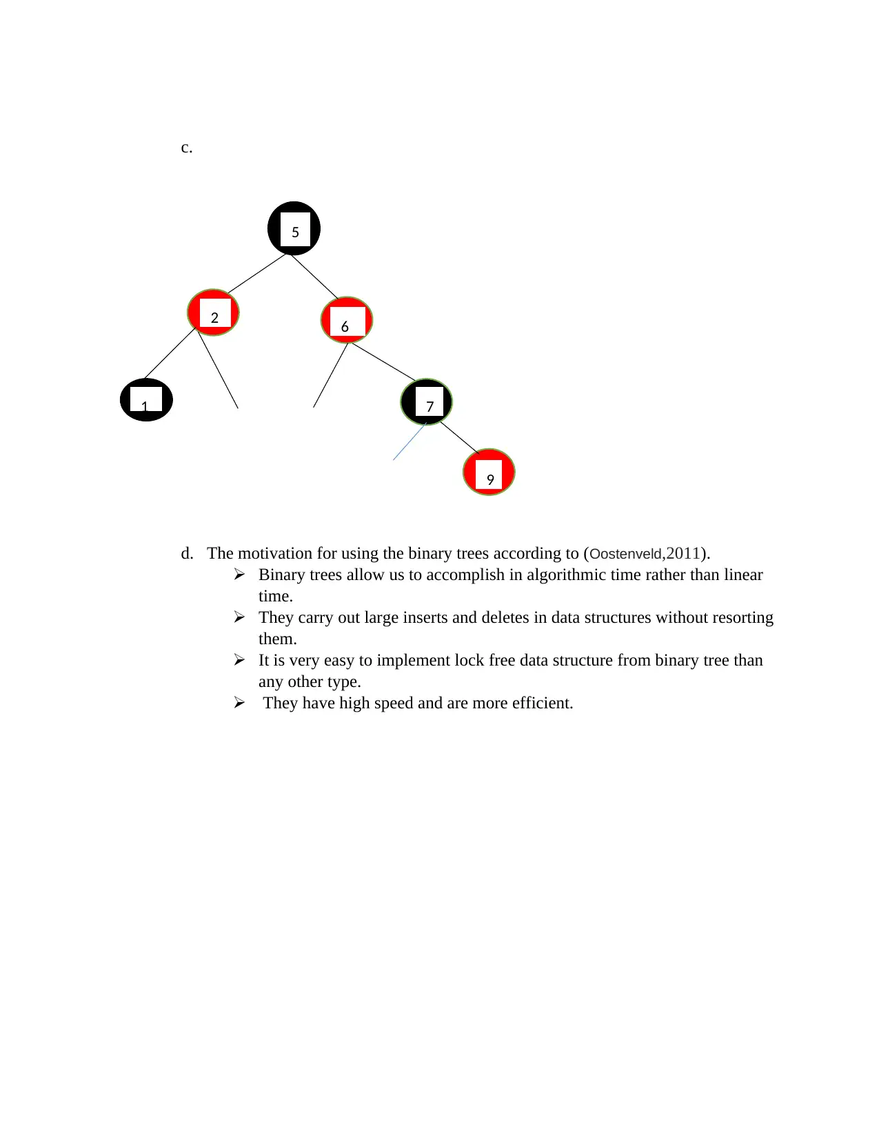
5
2 6
1 7
9

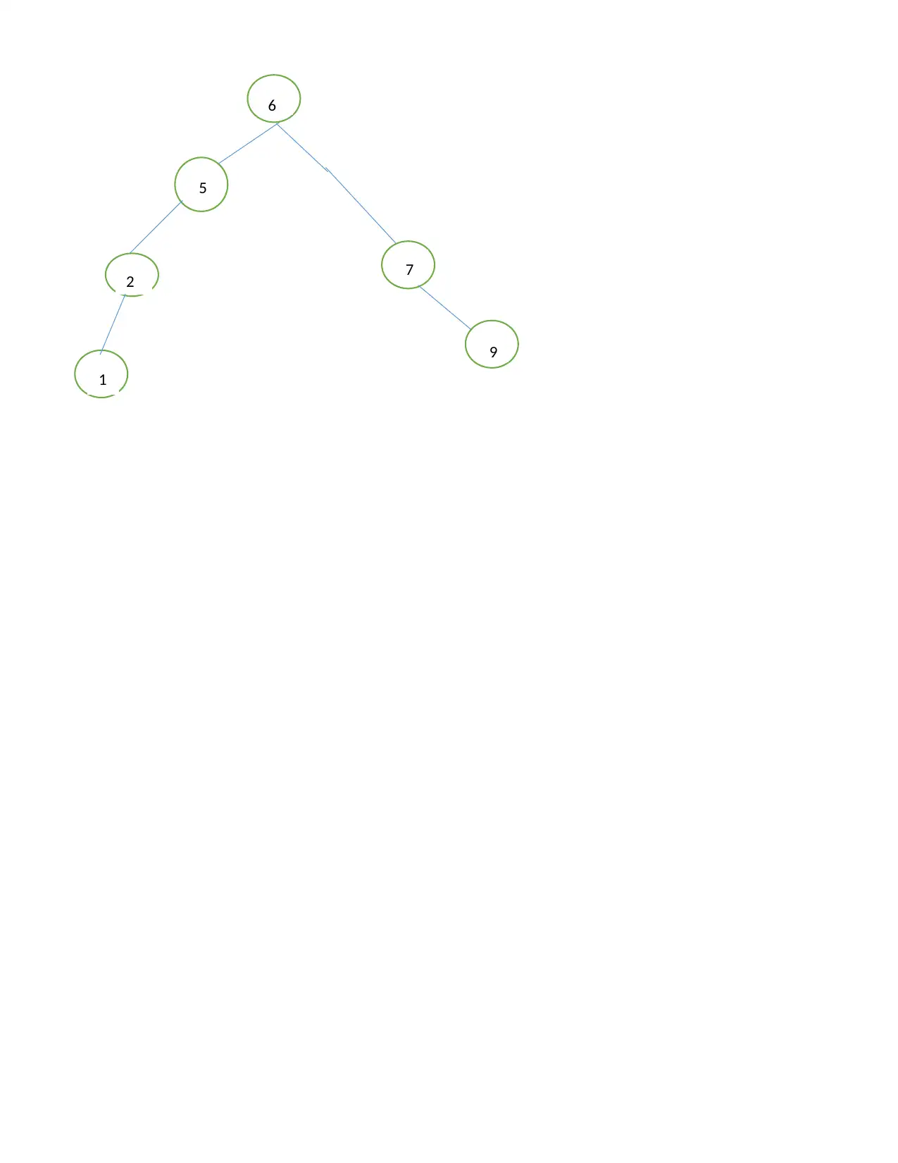
5
1
6
2 7
9

3.
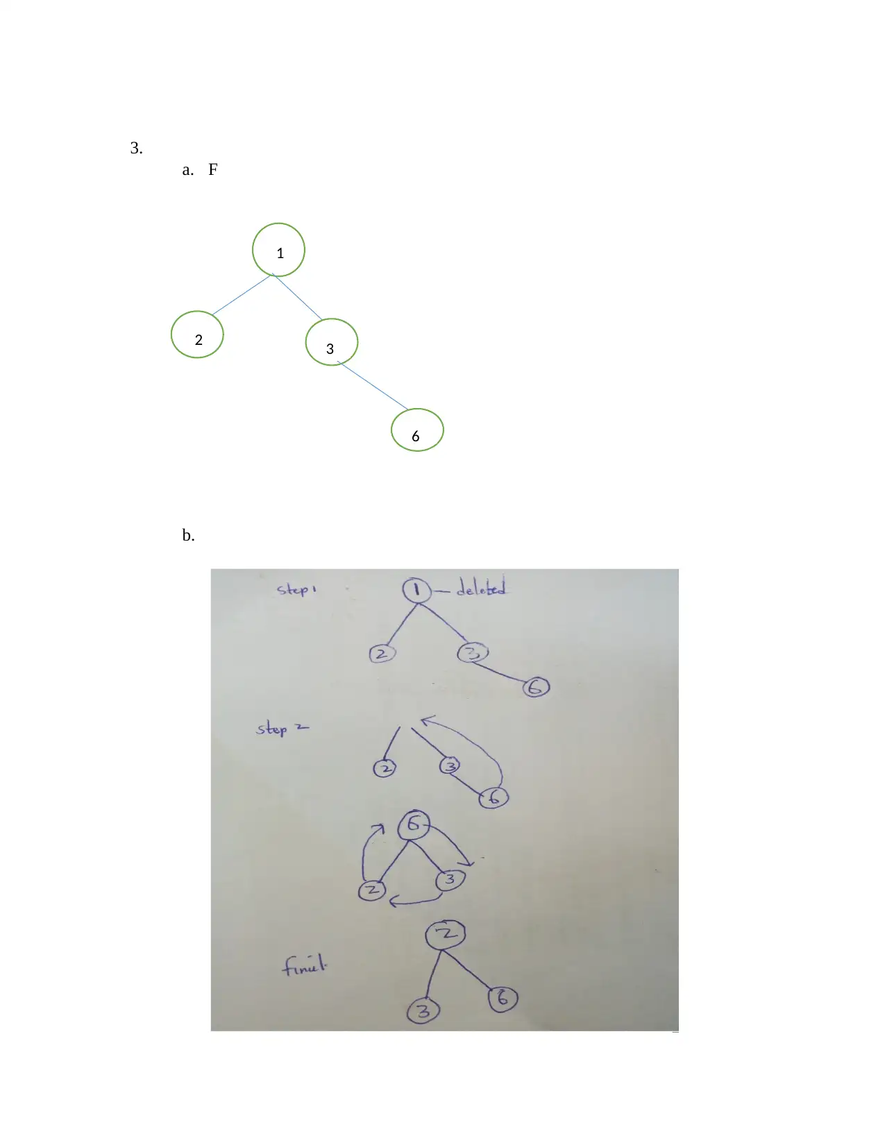
a. F
b.
1
2 3
6

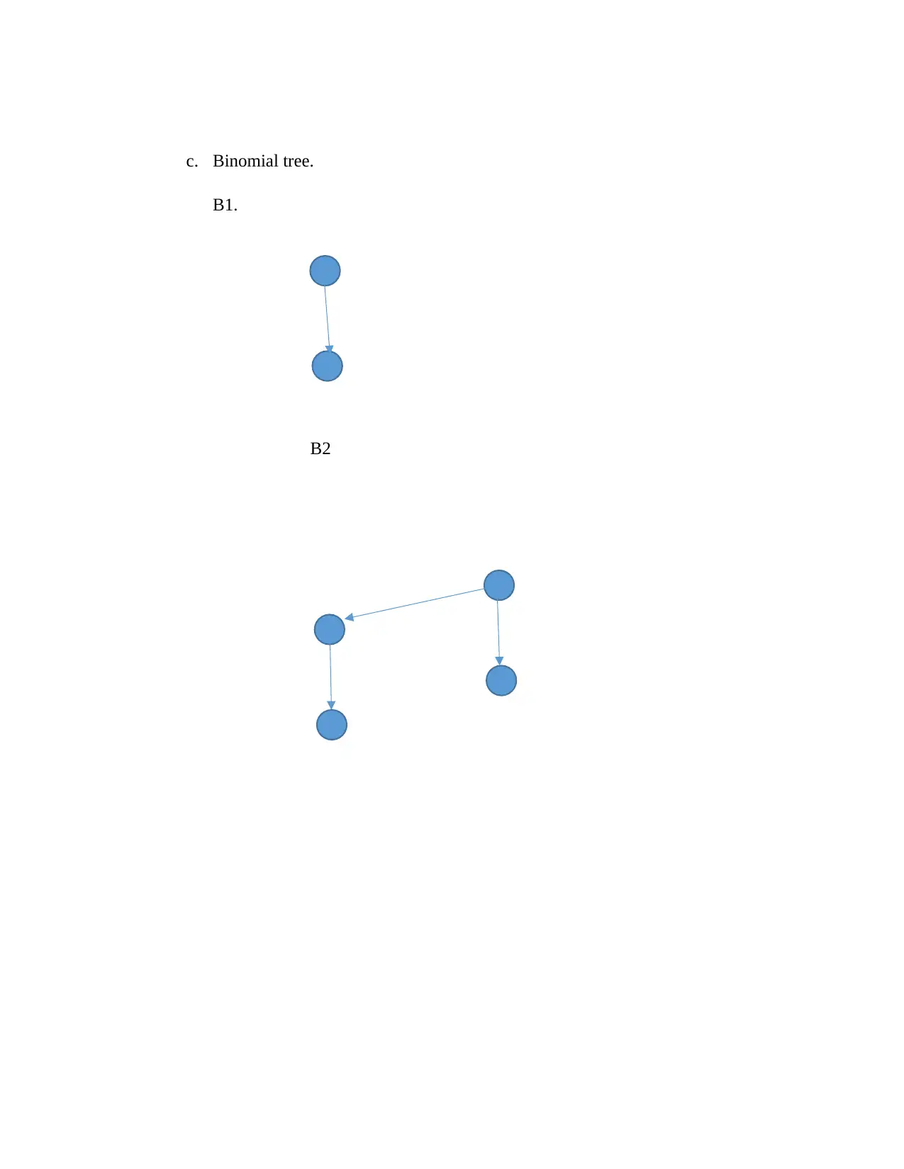
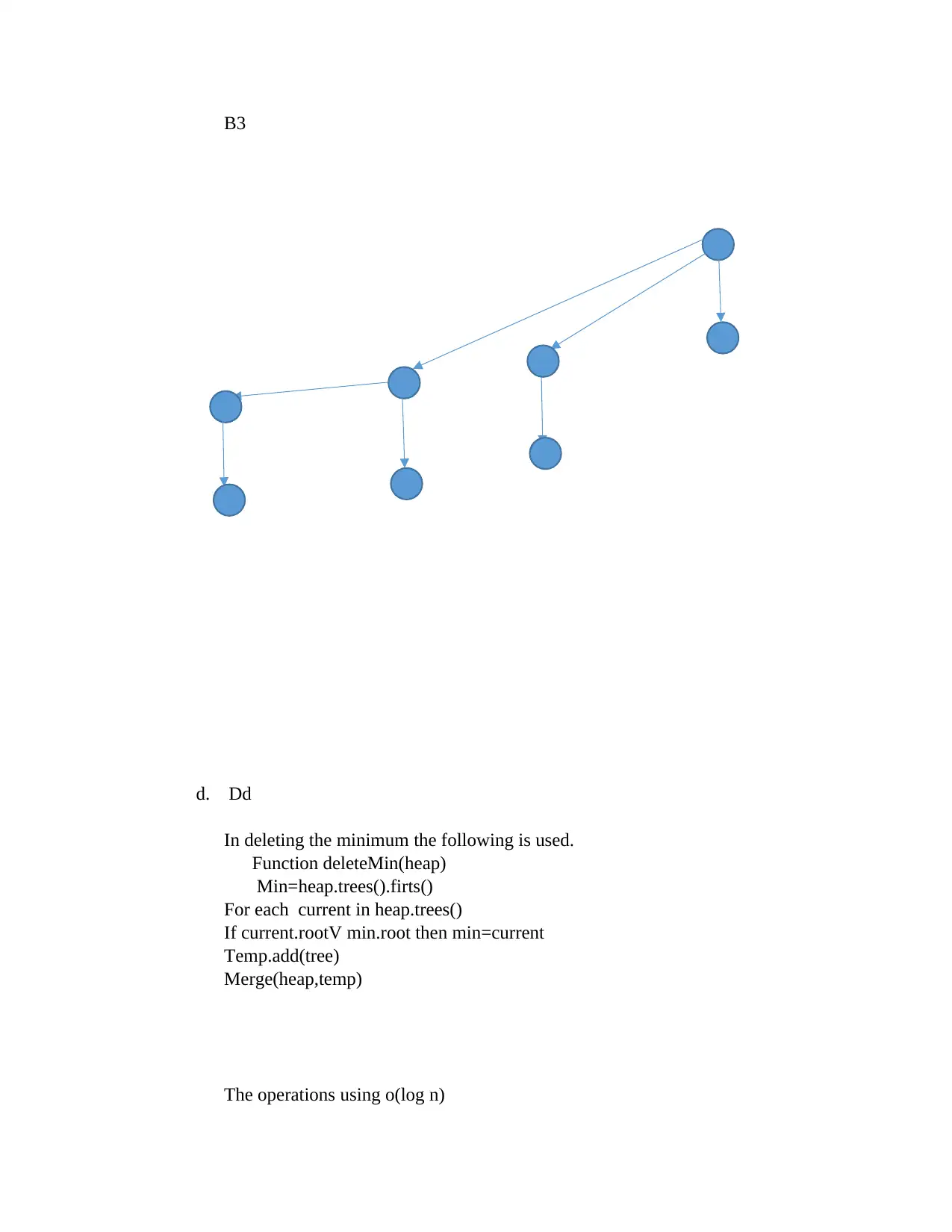
c. Binomial tree.
B1.
B2

B3
d. Dd
In deleting the minimum the following is used.
Function deleteMin(heap)
Min=heap.trees().firts()
For each current in heap.trees()
If current.rootV min.root then min=current
Temp.add(tree)
Merge(heap,temp)
The operations using o(log n)

4.
a.
The binary number search sort array takes 0(log n) because for any set of given
data the middle most element is the one that is checked first before the others. For
example if the large number is being looked for then the rest from the beginning
can be ignored (Abel,2014).
b. D
i. High>=low
ii. The mid is calculated=low +(high- low)/2
Return mid
iii. Else if(x>arr[mid])
Return first(arr,(mid+1),high,x,n);
iv. Else return first(arr,low(mid-1),x,n)
v. Otherwise return -1;
c.
 Describe the structure of an optimal arrangement of the vertices.
 The values of the parts are recursively defined and compared between the
vertexes and the optimum one is selected (Kiyok,2013).
 The values of the optimum solution are computed in bottom –up fashion.
 Then ideal arrangement which is the optimum solution is selected from
the recorded data.
 Then the recorded data are added to find the shortest route between the V1
and Vn

d.
e. To show that traveling salesman is NP-complete initial we verify NP belongs to
NP.if the tour contains all the vertexes and the calculated cost is minimum then
the then it belongs to TSp according to (Vitter,2012).
Proving than Tsp is hard is another step. By concluding that Hamiltonian cycle
≤p TSP
If it is assumed that
G = (V, E) are the instance of the Hamilton.
Then a complete graph can be created where
E′={(i,j):i,j∈Vandi≠j
If then G has a cost of at most 0 then its proven that traveling salesman is NP -
complete
1
1
1
1
2
2
1
1
3 4
2
1 2
V 1 V 3
V 4 V 6 V 7
V 0
V 8
V 5
V 2

Conclusion
Different kind of algorithms approach problems in different ways and solve them. Some
problems require to be divided into sub-problems in order to be solved, search cases require use
of dynamic programming algorithm. Best algorithm use the minimum time to solve a problem.

References
Abel, D. J., & Smith, J. L. (2014). A data structure and algorithm based on a linear key for a rectangle
retrieval problem. Computer Vision, Graphics, and Image Processing, 24(1), 1-13.
Berg, M. D., Cheong, O., Kreveld, M. V., & Overmars, M. (2008). Computational geometry: algorithms
and applications. Springer-Verlag TELOS.
Kiyoki, Y., Tanaka, K., Aiso, H., & Kamibayashi, N. (2013). Design and Evaluation of a Relational Data
Base Machine Employing Advanced Data Structures and Algorithms. In Conf Proc Annu Symp
Comput Archit 8th. IEEE Comput Soc Press.
Oostenveld, R., Fries, P., Maris, E., & Schoffelen, J. M. (2011). FieldTrip: open source software for
advanced analysis of MEG, EEG, and invasive electrophysiological data. Computational
intelligence and neuroscience, 2011, 1.
Vitter, J. S. (2012). External memory algorithms and data structures: Dealing with massive data. ACM
Computing surveys (CsUR), 33(2), 209-271.