Descriptive Statistics
VerifiedAdded on 2023/04/21
|19
|3583
|441
AI Summary
This document provides an explanation of descriptive statistics, including the construction of a frequency distribution table, histogram, and measures of central tendency and variability. It also discusses the context in which the data points represent a population or a sample.
Contribute Materials
Your contribution can guide someone’s learning journey. Share your
documents today.
Running Head: DESCRIPTIVE STATAISTICS
1
DESCRIPTIVE STATAISTICS
Name of student:
Name of Institution:
Date:
Author Note:
1
DESCRIPTIVE STATAISTICS
Name of student:
Name of Institution:
Date:
Author Note:
Secure Best Marks with AI Grader
Need help grading? Try our AI Grader for instant feedback on your assignments.
DESCRIPTIVE STATAISTICS
Psy2530- Problem Set #1
1) The data presented above could be considered a sample or population. Using the
information given in the introductory paragraph, explain to me in what context these 80
data points would represent a population and an example where they would represent a
sample.
Solution: The data represented above can be considered as a population if the study
involves a small group of individuals. For example, the investigation of the existence of
gender difference in the level of psychological well- being among the staff members of a
school. In the scenario of a staff member of a school, if the total number of staff members
in a school is 80, then the data set can be considered as a population. On the other hand, if
the investigation involves gender differences in a school with many students and staff
members, then the data set can be considered as a sample of the whole population in that
school. A sample is a subset of a population (Libman & Zipora, 2010)
2) a) What is the independent variable in this study?
Solution: The independent variable is gender (men or women).
b) What is the dependent variable? Is it a continuous or discrete variable? What is the
scale of measurement for this variable?
Solution: The dependent variable is the level of psychological well- being. The dependent
variable is continuous. The variable is measured on a numerical scale.
3) Construct a frequency distribution table with columns for a) absolute frequencies, b)
cumulative absolute frequencies and c) relative frequencies using all 80 data points.
Create a histogram illustrating the absolute frequencies. Be sure to calculate and
present all measures of central tendency and variability for this distribution, i.e., mean,
median, mode, range, variance, and standard deviation.
DESCRIPTIVE STATAISTICS
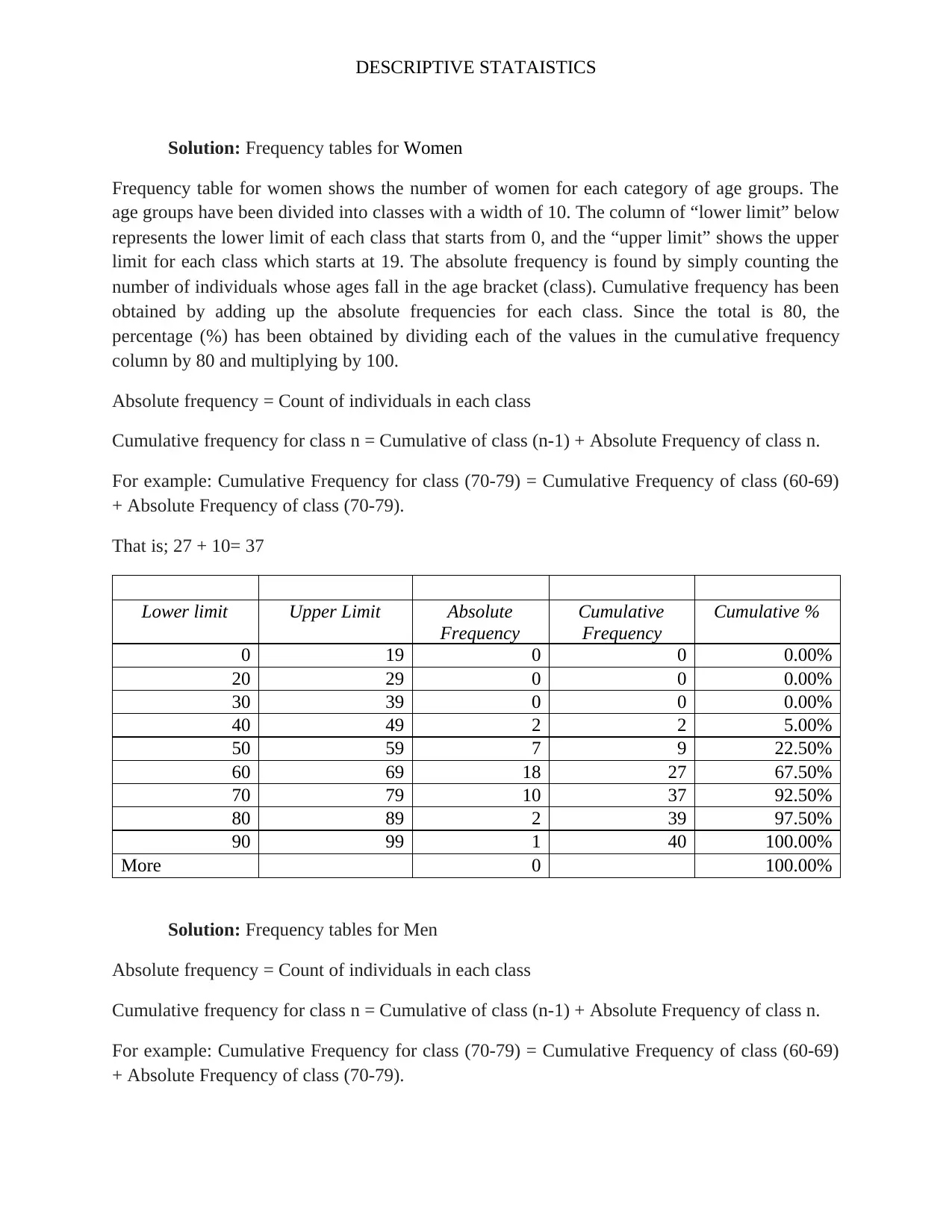
Solution: Frequency tables for Women
Frequency table for women shows the number of women for each category of age groups. The
age groups have been divided into classes with a width of 10. The column of “lower limit” below
represents the lower limit of each class that starts from 0, and the “upper limit” shows the upper
limit for each class which starts at 19. The absolute frequency is found by simply counting the
number of individuals whose ages fall in the age bracket (class). Cumulative frequency has been
obtained by adding up the absolute frequencies for each class. Since the total is 80, the
percentage (%) has been obtained by dividing each of the values in the cumulative frequency
column by 80 and multiplying by 100.
Absolute frequency = Count of individuals in each class
Cumulative frequency for class n = Cumulative of class (n-1) + Absolute Frequency of class n.
For example: Cumulative Frequency for class (70-79) = Cumulative Frequency of class (60-69)
+ Absolute Frequency of class (70-79).
That is; 27 + 10= 37
Lower limit Upper Limit Absolute
Frequency
Cumulative
Frequency
Cumulative %
0 19 0 0 0.00%
20 29 0 0 0.00%
30 39 0 0 0.00%
40 49 2 2 5.00%
50 59 7 9 22.50%
60 69 18 27 67.50%
70 79 10 37 92.50%
80 89 2 39 97.50%
90 99 1 40 100.00%
More 0 100.00%
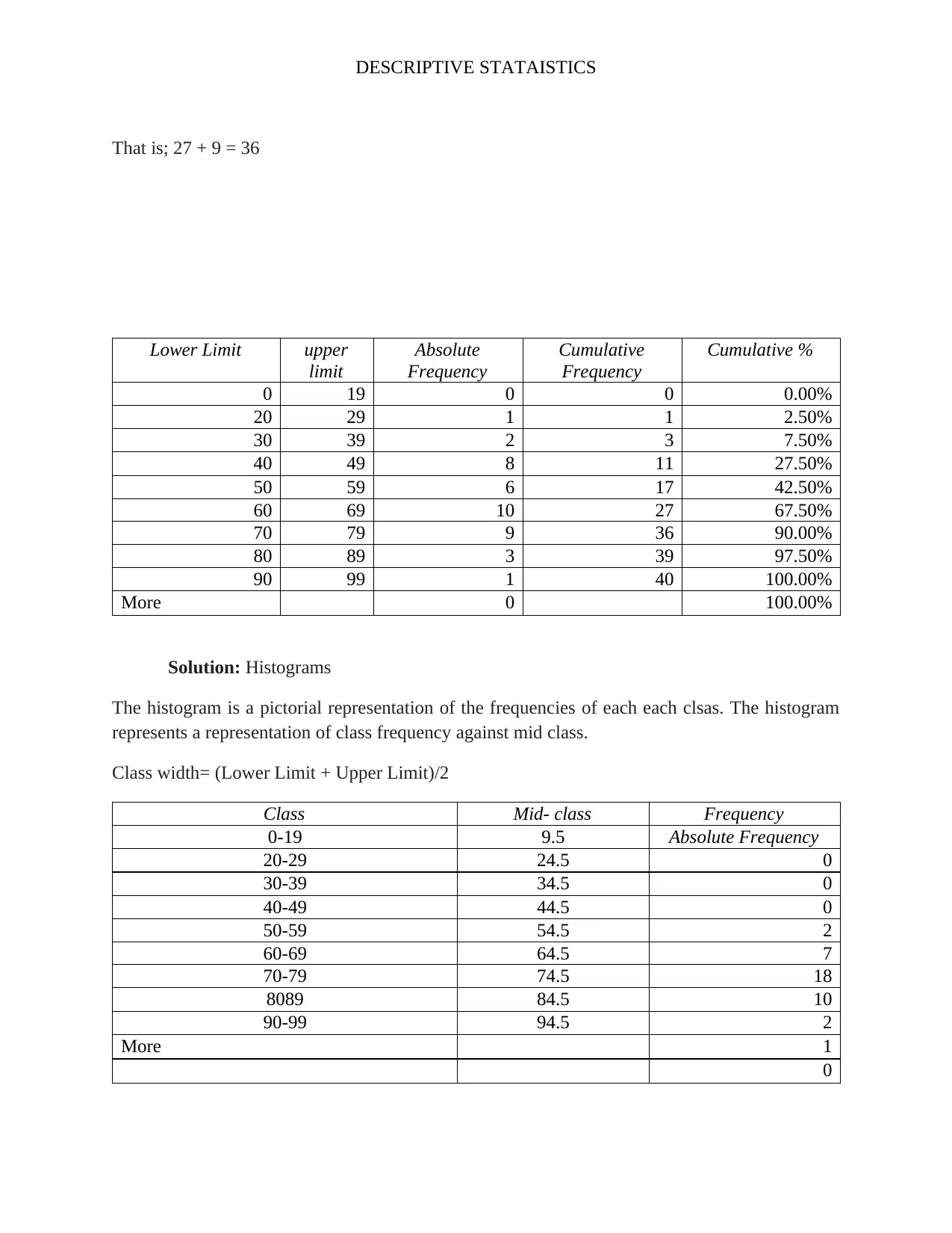
Solution: Frequency tables for Men
Absolute frequency = Count of individuals in each class
Cumulative frequency for class n = Cumulative of class (n-1) + Absolute Frequency of class n.
For example: Cumulative Frequency for class (70-79) = Cumulative Frequency of class (60-69)
+ Absolute Frequency of class (70-79).
DESCRIPTIVE STATAISTICS
That is; 27 + 9 = 36
Lower Limit upper
limit
Absolute
Frequency
Cumulative
Frequency
Cumulative %
0 19 0 0 0.00%
20 29 1 1 2.50%
30 39 2 3 7.50%
40 49 8 11 27.50%
50 59 6 17 42.50%
60 69 10 27 67.50%
70 79 9 36 90.00%
80 89 3 39 97.50%
90 99 1 40 100.00%
More 0 100.00%
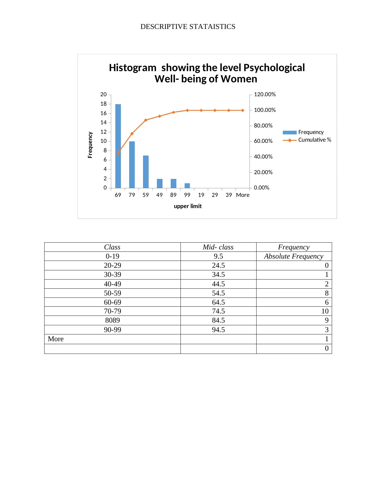
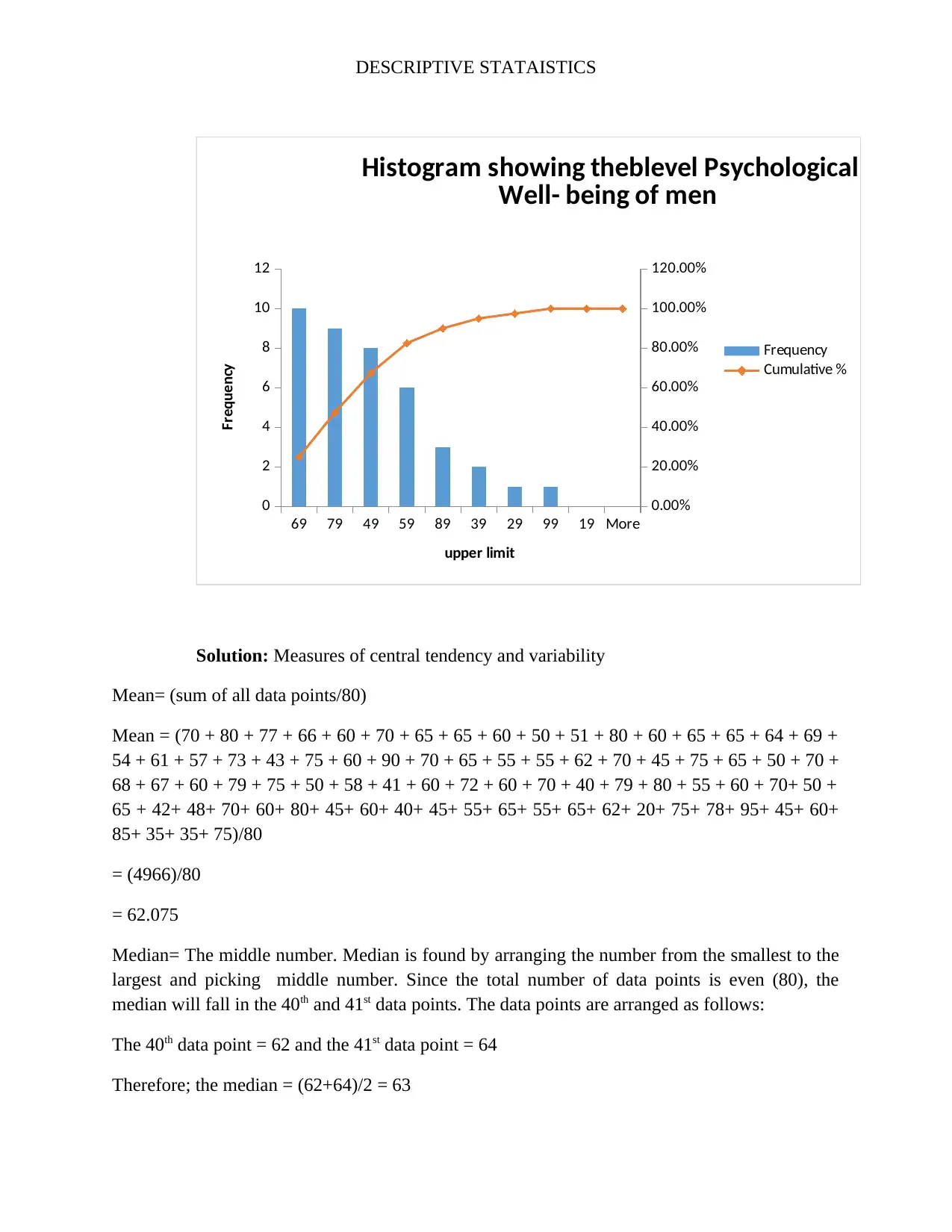
Solution: Histograms
The histogram is a pictorial representation of the frequencies of each each clsas. The histogram
represents a representation of class frequency against mid class.
Class width= (Lower Limit + Upper Limit)/2
Class Mid- class Frequency
0-19 9.5 Absolute Frequency
20-29 24.5 0
30-39 34.5 0
40-49 44.5 0
50-59 54.5 2
60-69 64.5 7
70-79 74.5 18
8089 84.5 10
90-99 94.5 2
More 1
0
Paraphrase This Document
Need a fresh take? Get an instant paraphrase of this document with our AI Paraphraser
DESCRIPTIVE STATAISTICS
69 79 59 49 89 99 19 29 39 More
0
2
4
6
8
10
12
14
16
18
20
0.00%
20.00%
40.00%
60.00%
80.00%
100.00%
120.00%
Histogram showing the level Psychological
Well- being of Women
Frequency
Cumulative %
upper limit
Frequency
Class Mid- class Frequency
0-19 9.5 Absolute Frequency
20-29 24.5 0
30-39 34.5 1
40-49 44.5 2
50-59 54.5 8
60-69 64.5 6
70-79 74.5 10
8089 84.5 9
90-99 94.5 3
More 1
0
DESCRIPTIVE STATAISTICS
69 79 49 59 89 39 29 99 19 More
0
2
4
6
8
10
12
0.00%
20.00%
40.00%
60.00%
80.00%
100.00%
120.00%
Histogram showing theblevel Psychological
Well- being of men
Frequency
Cumulative %
upper limit
Frequency
Solution: Measures of central tendency and variability
Mean= (sum of all data points/80)
Mean = (70 + 80 + 77 + 66 + 60 + 70 + 65 + 65 + 60 + 50 + 51 + 80 + 60 + 65 + 65 + 64 + 69 +
54 + 61 + 57 + 73 + 43 + 75 + 60 + 90 + 70 + 65 + 55 + 55 + 62 + 70 + 45 + 75 + 65 + 50 + 70 +
68 + 67 + 60 + 79 + 75 + 50 + 58 + 41 + 60 + 72 + 60 + 70 + 40 + 79 + 80 + 55 + 60 + 70+ 50 +
65 + 42+ 48+ 70+ 60+ 80+ 45+ 60+ 40+ 45+ 55+ 65+ 55+ 65+ 62+ 20+ 75+ 78+ 95+ 45+ 60+
85+ 35+ 35+ 75)/80
= (4966)/80
= 62.075
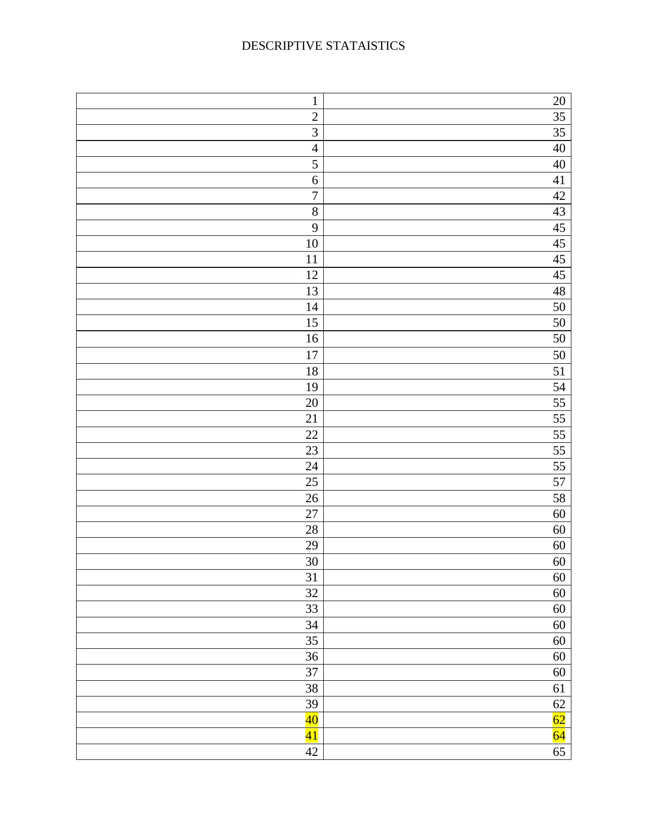
Median= The middle number. Median is found by arranging the number from the smallest to the
largest and picking middle number. Since the total number of data points is even (80), the
median will fall in the 40th and 41st data points. The data points are arranged as follows:
The 40th data point = 62 and the 41st data point = 64
Therefore; the median = (62+64)/2 = 63

DESCRIPTIVE STATAISTICS
Position Data point
Position Data point
Secure Best Marks with AI Grader
Need help grading? Try our AI Grader for instant feedback on your assignments.
DESCRIPTIVE STATAISTICS
1 20
2 35
3 35
4 40
5 40
6 41
7 42
8 43
9 45
10 45
11 45
12 45
13 48
14 50
15 50
16 50
17 50
18 51
19 54
20 55
21 55
22 55
23 55
24 55
25 57
26 58
27 60
28 60
29 60
30 60
31 60
32 60
33 60
34 60
35 60
36 60
37 60
38 61
39 62
40 62
41 64
42 65
1 20
2 35
3 35
4 40
5 40
6 41
7 42
8 43
9 45
10 45
11 45
12 45
13 48
14 50
15 50
16 50
17 50
18 51
19 54
20 55
21 55
22 55
23 55
24 55
25 57
26 58
27 60
28 60
29 60
30 60
31 60
32 60
33 60
34 60
35 60
36 60
37 60
38 61
39 62
40 62
41 64
42 65
DESCRIPTIVE STATAISTICS
43 65
44 65
45 65
46 65
47 65
48 65
49 65
50 65
51 66
52 67
53 68
54 69
55 70
56 70
57 70
58 70
59 70
60 70
61 70
62 70
63 72
64 73
65 75
66 75
67 75
68 75
69 75
70 77
71 78
72 79
73 79
74 80
75 80
76 80
77 80
78 85
79 90
80 95
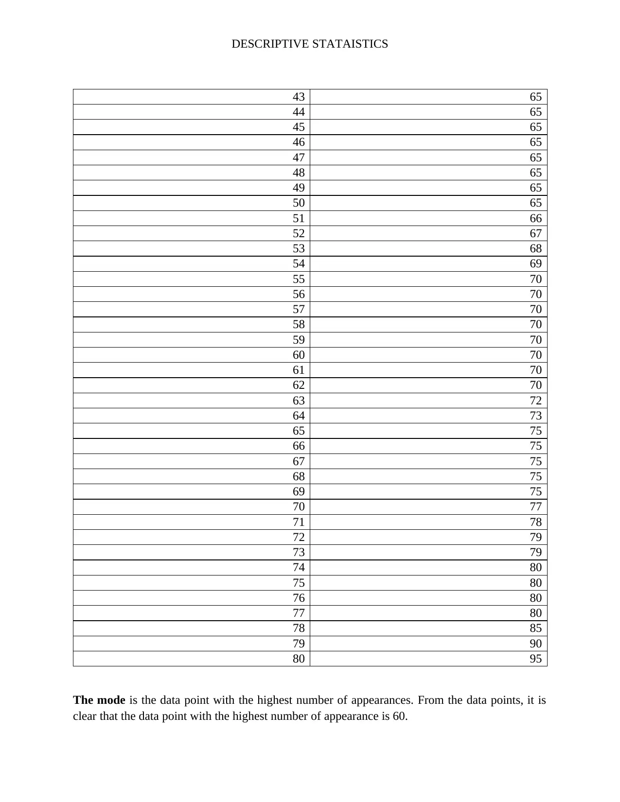
The mode is the data point with the highest number of appearances. From the data points, it is
clear that the data point with the highest number of appearance is 60.
DESCRIPTIVE STATAISTICS
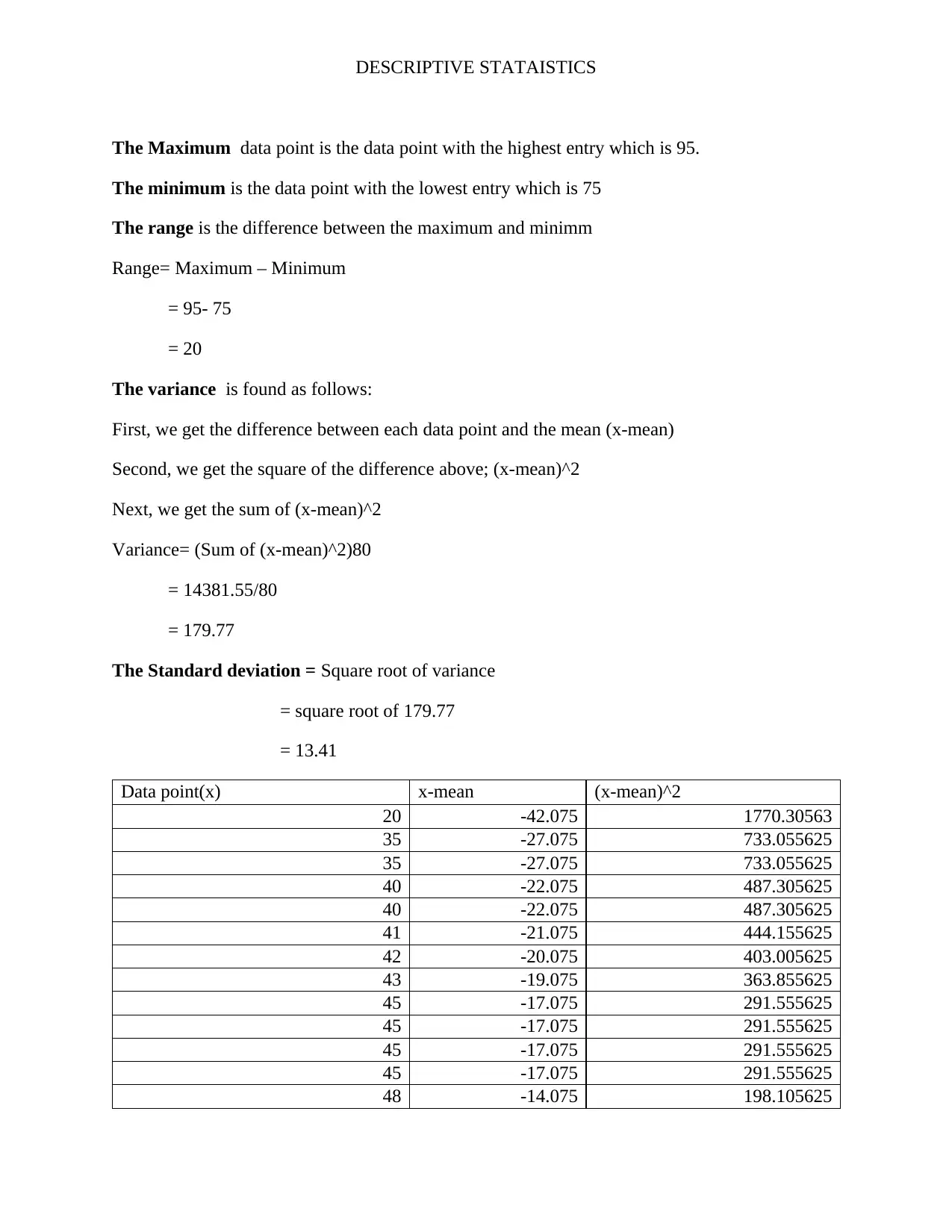
The Maximum data point is the data point with the highest entry which is 95.
The minimum is the data point with the lowest entry which is 75
The range is the difference between the maximum and minimm
Range= Maximum – Minimum
= 95- 75
= 20
The variance is found as follows:
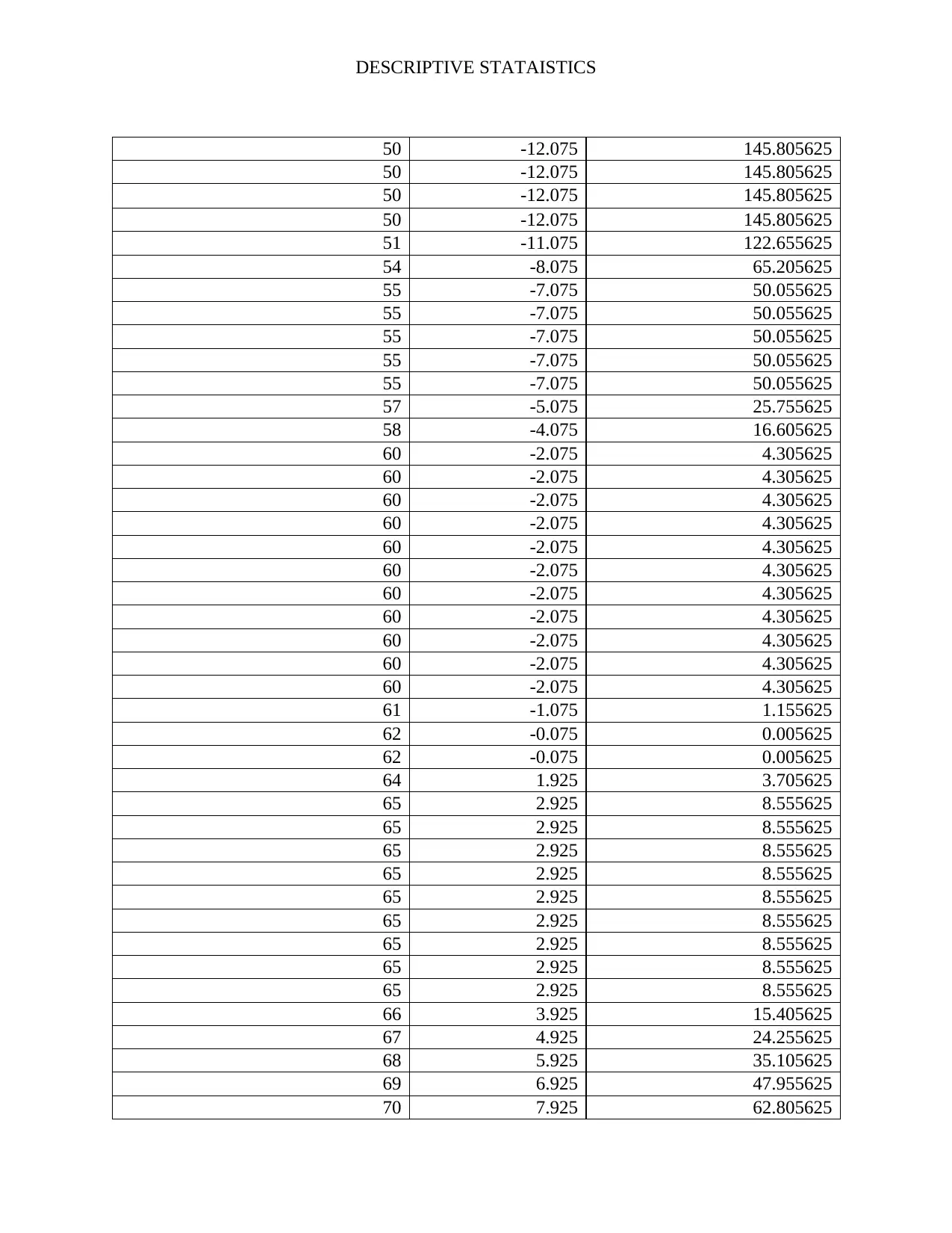
First, we get the difference between each data point and the mean (x-mean)
Second, we get the square of the difference above; (x-mean)^2
Next, we get the sum of (x-mean)^2
Variance= (Sum of (x-mean)^2)80
= 14381.55/80
= 179.77
The Standard deviation = Square root of variance
= square root of 179.77
= 13.41
Data point(x) x-mean (x-mean)^2
20 -42.075 1770.30563
35 -27.075 733.055625
35 -27.075 733.055625
40 -22.075 487.305625
40 -22.075 487.305625
41 -21.075 444.155625
42 -20.075 403.005625
43 -19.075 363.855625
45 -17.075 291.555625
45 -17.075 291.555625
45 -17.075 291.555625
45 -17.075 291.555625
48 -14.075 198.105625
Paraphrase This Document
Need a fresh take? Get an instant paraphrase of this document with our AI Paraphraser
DESCRIPTIVE STATAISTICS
50 -12.075 145.805625
50 -12.075 145.805625
50 -12.075 145.805625
50 -12.075 145.805625
51 -11.075 122.655625
54 -8.075 65.205625
55 -7.075 50.055625
55 -7.075 50.055625
55 -7.075 50.055625
55 -7.075 50.055625
55 -7.075 50.055625
57 -5.075 25.755625
58 -4.075 16.605625
60 -2.075 4.305625
60 -2.075 4.305625
60 -2.075 4.305625
60 -2.075 4.305625
60 -2.075 4.305625
60 -2.075 4.305625
60 -2.075 4.305625
60 -2.075 4.305625
60 -2.075 4.305625
60 -2.075 4.305625
60 -2.075 4.305625
61 -1.075 1.155625
62 -0.075 0.005625
62 -0.075 0.005625
64 1.925 3.705625
65 2.925 8.555625
65 2.925 8.555625
65 2.925 8.555625
65 2.925 8.555625
65 2.925 8.555625
65 2.925 8.555625
65 2.925 8.555625
65 2.925 8.555625
65 2.925 8.555625
66 3.925 15.405625
67 4.925 24.255625
68 5.925 35.105625
69 6.925 47.955625
70 7.925 62.805625
50 -12.075 145.805625
50 -12.075 145.805625
50 -12.075 145.805625
50 -12.075 145.805625
51 -11.075 122.655625
54 -8.075 65.205625
55 -7.075 50.055625
55 -7.075 50.055625
55 -7.075 50.055625
55 -7.075 50.055625
55 -7.075 50.055625
57 -5.075 25.755625
58 -4.075 16.605625
60 -2.075 4.305625
60 -2.075 4.305625
60 -2.075 4.305625
60 -2.075 4.305625
60 -2.075 4.305625
60 -2.075 4.305625
60 -2.075 4.305625
60 -2.075 4.305625
60 -2.075 4.305625
60 -2.075 4.305625
60 -2.075 4.305625
61 -1.075 1.155625
62 -0.075 0.005625
62 -0.075 0.005625
64 1.925 3.705625
65 2.925 8.555625
65 2.925 8.555625
65 2.925 8.555625
65 2.925 8.555625
65 2.925 8.555625
65 2.925 8.555625
65 2.925 8.555625
65 2.925 8.555625
65 2.925 8.555625
66 3.925 15.405625
67 4.925 24.255625
68 5.925 35.105625
69 6.925 47.955625
70 7.925 62.805625
DESCRIPTIVE STATAISTICS
70 7.925 62.805625
70 7.925 62.805625
70 7.925 62.805625
70 7.925 62.805625
70 7.925 62.805625
70 7.925 62.805625
70 7.925 62.805625
72 9.925 98.505625
73 10.925 119.355625
75 12.925 167.055625
75 12.925 167.055625
75 12.925 167.055625
75 12.925 167.055625
75 12.925 167.055625
77 14.925 222.755625
78 15.925 253.605625
79 16.925 286.455625
79 16.925 286.455625
80 17.925 321.305625
80 17.925 321.305625
80 17.925 321.305625
80 17.925 321.305625
85 22.925 525.555625
90 27.925 779.805625
95 32.925 1084.05563
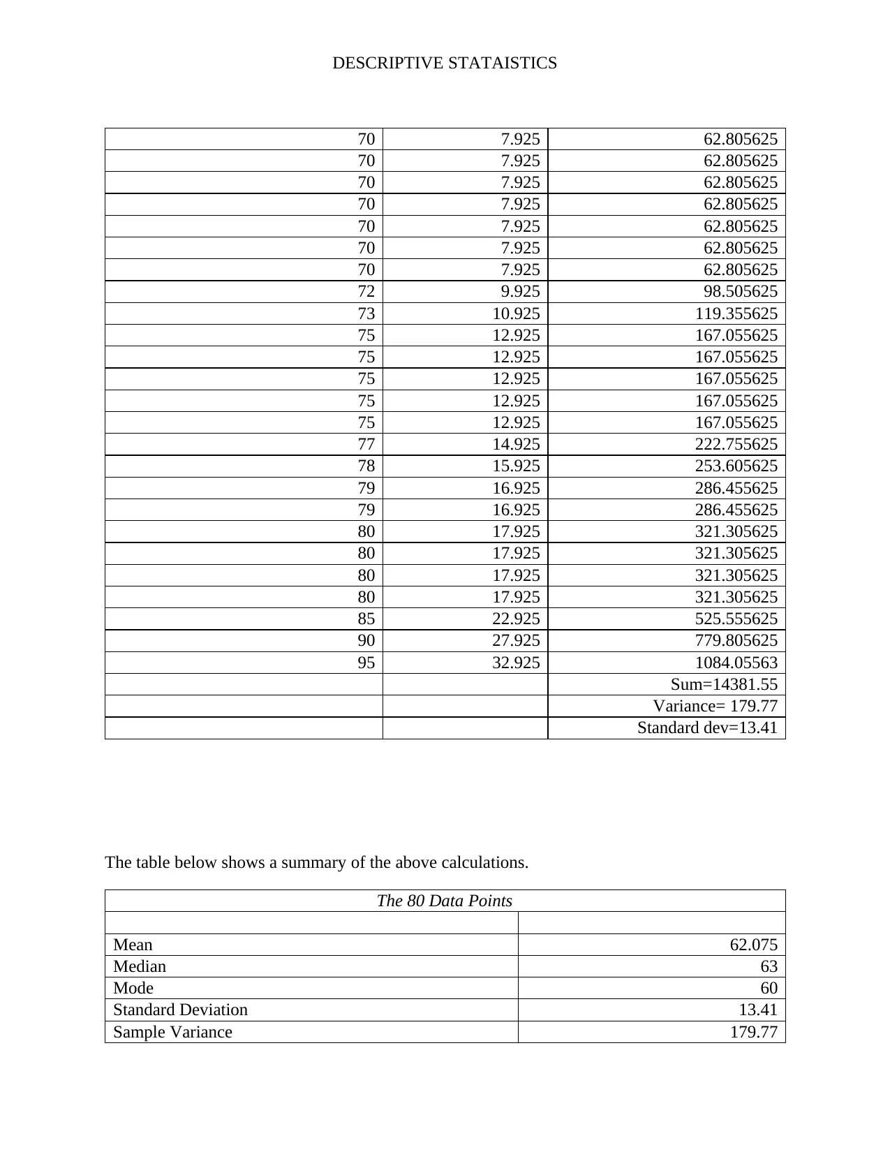
Sum=14381.55
Variance= 179.77
Standard dev=13.41
The table below shows a summary of the above calculations.
The 80 Data Points
Mean 62.075
Median 63
Mode 60
Standard Deviation 13.41
Sample Variance 179.77
70 7.925 62.805625
70 7.925 62.805625
70 7.925 62.805625
70 7.925 62.805625
70 7.925 62.805625
70 7.925 62.805625
70 7.925 62.805625
72 9.925 98.505625
73 10.925 119.355625
75 12.925 167.055625
75 12.925 167.055625
75 12.925 167.055625
75 12.925 167.055625
75 12.925 167.055625
77 14.925 222.755625
78 15.925 253.605625
79 16.925 286.455625
79 16.925 286.455625
80 17.925 321.305625
80 17.925 321.305625
80 17.925 321.305625
80 17.925 321.305625
85 22.925 525.555625
90 27.925 779.805625
95 32.925 1084.05563
Sum=14381.55
Variance= 179.77
Standard dev=13.41
The table below shows a summary of the above calculations.
The 80 Data Points
Mean 62.075
Median 63
Mode 60
Standard Deviation 13.41
Sample Variance 179.77
DESCRIPTIVE STATAISTICS
Range 75
Minimum 20
Maximum 95
Sum 4966
Count 80
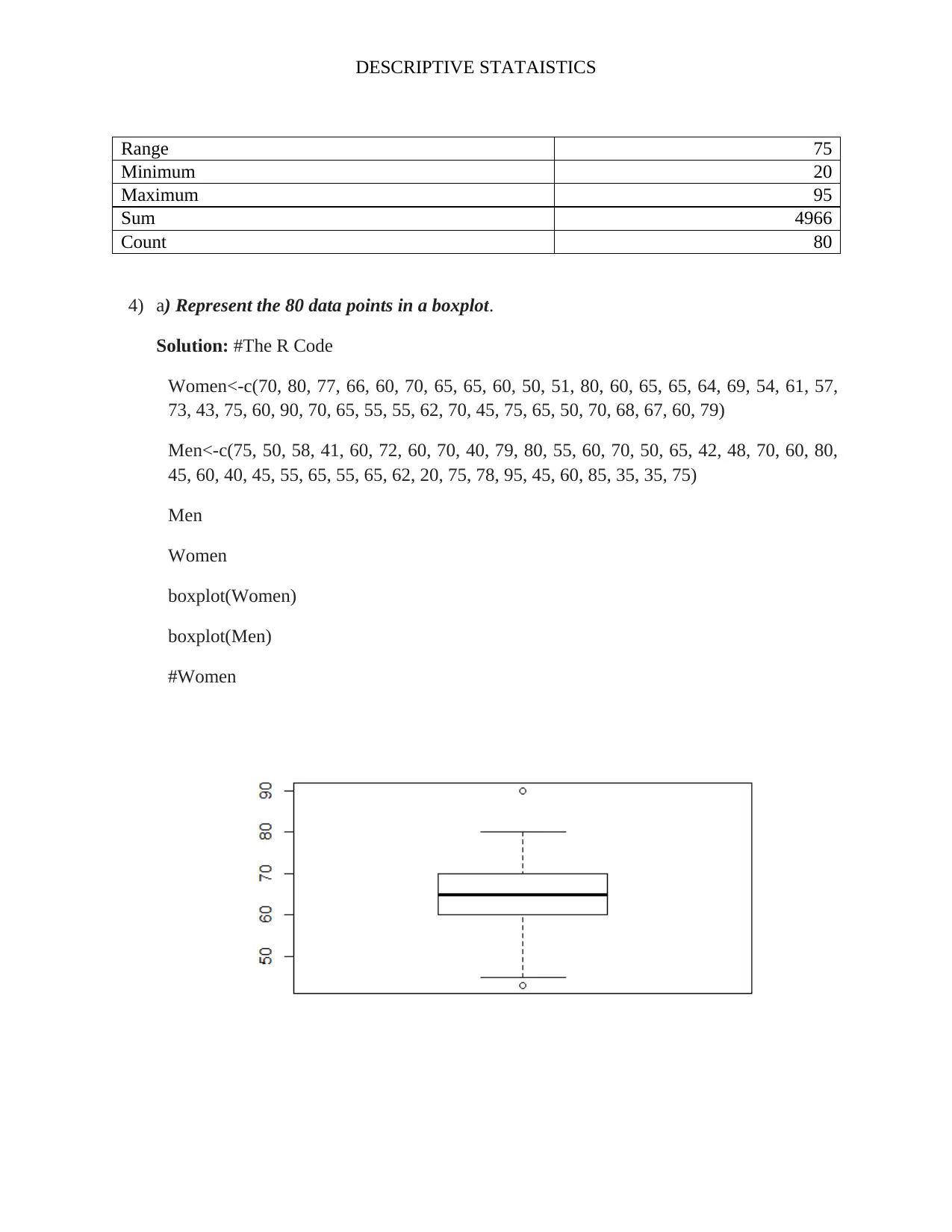
4) a) Represent the 80 data points in a boxplot.
Solution: #The R Code
Women<-c(70, 80, 77, 66, 60, 70, 65, 65, 60, 50, 51, 80, 60, 65, 65, 64, 69, 54, 61, 57,
73, 43, 75, 60, 90, 70, 65, 55, 55, 62, 70, 45, 75, 65, 50, 70, 68, 67, 60, 79)
Men<-c(75, 50, 58, 41, 60, 72, 60, 70, 40, 79, 80, 55, 60, 70, 50, 65, 42, 48, 70, 60, 80,
45, 60, 40, 45, 55, 65, 55, 65, 62, 20, 75, 78, 95, 45, 60, 85, 35, 35, 75)
Men
Women
boxplot(Women)
boxplot(Men)
#Women
Secure Best Marks with AI Grader
Need help grading? Try our AI Grader for instant feedback on your assignments.
DESCRIPTIVE STATAISTICS
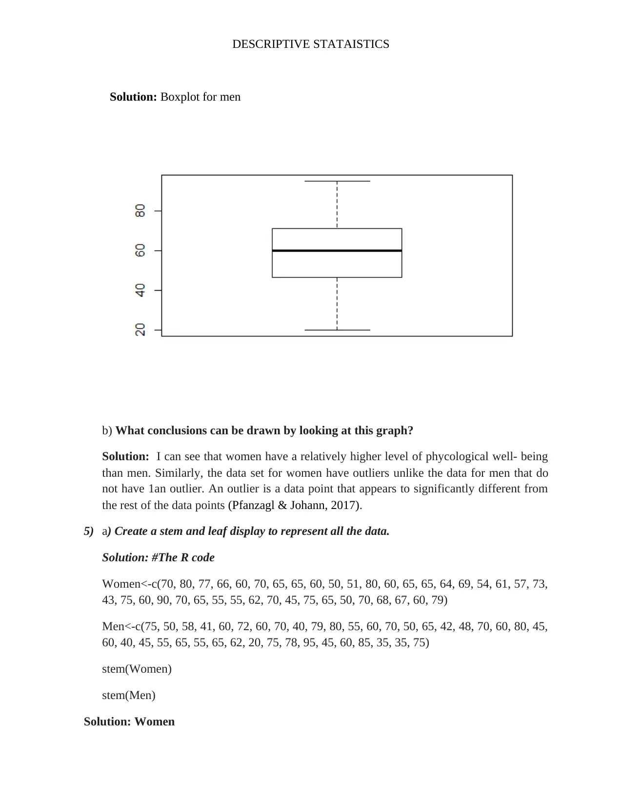
Solution: Boxplot for men
b) What conclusions can be drawn by looking at this graph?
Solution: I can see that women have a relatively higher level of phycological well- being
than men. Similarly, the data set for women have outliers unlike the data for men that do
not have 1an outlier. An outlier is a data point that appears to significantly different from
the rest of the data points (Pfanzagl & Johann, 2017).
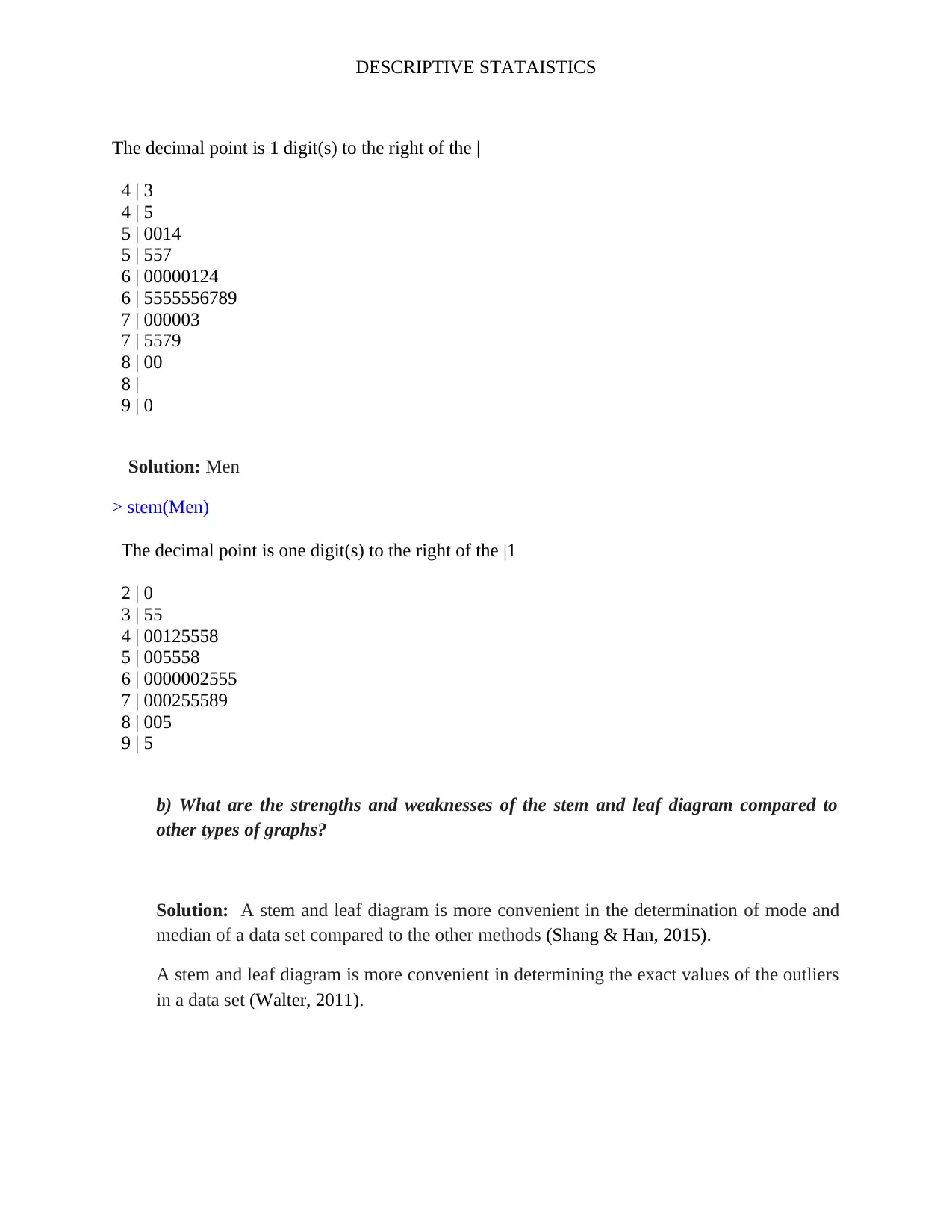
5) a) Create a stem and leaf display to represent all the data.
Solution: #The R code
Women<-c(70, 80, 77, 66, 60, 70, 65, 65, 60, 50, 51, 80, 60, 65, 65, 64, 69, 54, 61, 57, 73,
43, 75, 60, 90, 70, 65, 55, 55, 62, 70, 45, 75, 65, 50, 70, 68, 67, 60, 79)
Men<-c(75, 50, 58, 41, 60, 72, 60, 70, 40, 79, 80, 55, 60, 70, 50, 65, 42, 48, 70, 60, 80, 45,
60, 40, 45, 55, 65, 55, 65, 62, 20, 75, 78, 95, 45, 60, 85, 35, 35, 75)
stem(Women)
stem(Men)
Solution: Women
DESCRIPTIVE STATAISTICS
The decimal point is 1 digit(s) to the right of the |
4 | 3
4 | 5
5 | 0014
5 | 557
6 | 00000124
6 | 5555556789
7 | 000003
7 | 5579
8 | 00
8 |
9 | 0
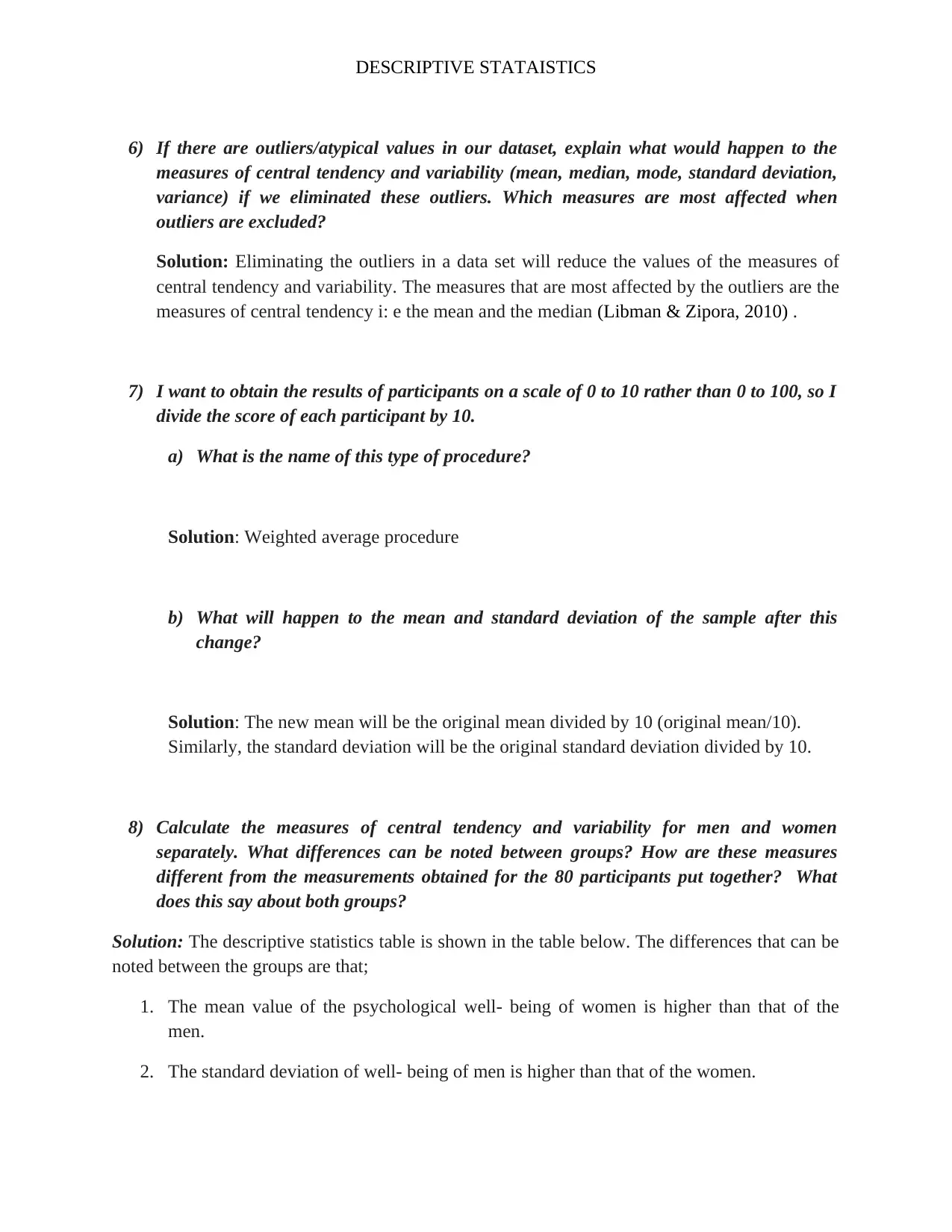
Solution: Men
> stem(Men)
The decimal point is one digit(s) to the right of the |1
2 | 0
3 | 55
4 | 00125558
5 | 005558
6 | 0000002555
7 | 000255589
8 | 005
9 | 5
b) What are the strengths and weaknesses of the stem and leaf diagram compared to
other types of graphs?
Solution: A stem and leaf diagram is more convenient in the determination of mode and
median of a data set compared to the other methods (Shang & Han, 2015).
A stem and leaf diagram is more convenient in determining the exact values of the outliers
in a data set (Walter, 2011).
DESCRIPTIVE STATAISTICS
6) If there are outliers/atypical values in our dataset, explain what would happen to the
measures of central tendency and variability (mean, median, mode, standard deviation,
variance) if we eliminated these outliers. Which measures are most affected when
outliers are excluded?
Solution: Eliminating the outliers in a data set will reduce the values of the measures of
central tendency and variability. The measures that are most affected by the outliers are the
measures of central tendency i: e the mean and the median (Libman & Zipora, 2010) .
7) I want to obtain the results of participants on a scale of 0 to 10 rather than 0 to 100, so I
divide the score of each participant by 10.
a) What is the name of this type of procedure?
Solution: Weighted average procedure
b) What will happen to the mean and standard deviation of the sample after this
change?
Solution: The new mean will be the original mean divided by 10 (original mean/10).
Similarly, the standard deviation will be the original standard deviation divided by 10.
8) Calculate the measures of central tendency and variability for men and women
separately. What differences can be noted between groups? How are these measures
different from the measurements obtained for the 80 participants put together? What
does this say about both groups?
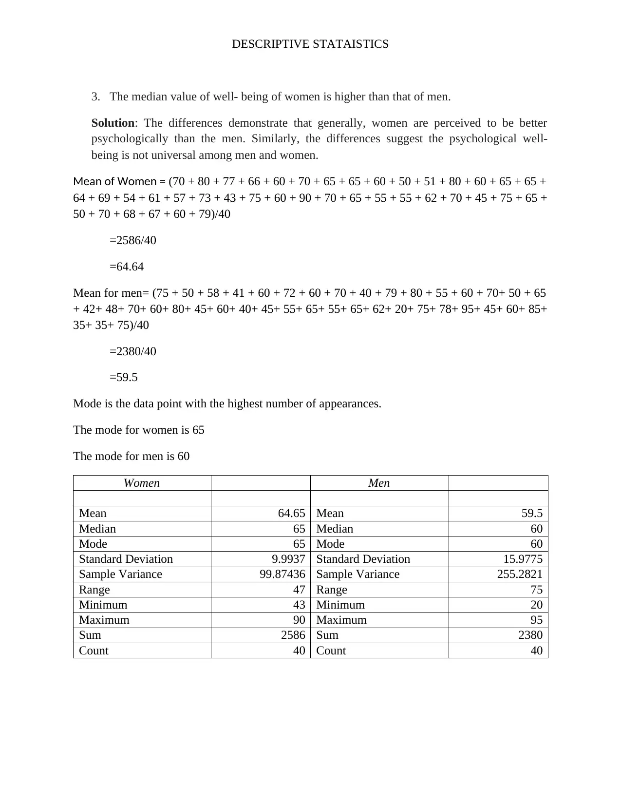
Solution: The descriptive statistics table is shown in the table below. The differences that can be
noted between the groups are that;
1. The mean value of the psychological well- being of women is higher than that of the
men.
2. The standard deviation of well- being of men is higher than that of the women.
Paraphrase This Document
Need a fresh take? Get an instant paraphrase of this document with our AI Paraphraser
DESCRIPTIVE STATAISTICS
3. The median value of well- being of women is higher than that of men.
Solution: The differences demonstrate that generally, women are perceived to be better
psychologically than the men. Similarly, the differences suggest the psychological well-
being is not universal among men and women.
Mean of Women = (70 + 80 + 77 + 66 + 60 + 70 + 65 + 65 + 60 + 50 + 51 + 80 + 60 + 65 + 65 +
64 + 69 + 54 + 61 + 57 + 73 + 43 + 75 + 60 + 90 + 70 + 65 + 55 + 55 + 62 + 70 + 45 + 75 + 65 +
50 + 70 + 68 + 67 + 60 + 79)/40
=2586/40
=64.64
Mean for men= (75 + 50 + 58 + 41 + 60 + 72 + 60 + 70 + 40 + 79 + 80 + 55 + 60 + 70+ 50 + 65
+ 42+ 48+ 70+ 60+ 80+ 45+ 60+ 40+ 45+ 55+ 65+ 55+ 65+ 62+ 20+ 75+ 78+ 95+ 45+ 60+ 85+
35+ 35+ 75)/40
=2380/40
=59.5
Mode is the data point with the highest number of appearances.
The mode for women is 65
The mode for men is 60
Women Men
Mean 64.65 Mean 59.5
Median 65 Median 60
Mode 65 Mode 60
Standard Deviation 9.9937 Standard Deviation 15.9775
Sample Variance 99.87436 Sample Variance 255.2821
Range 47 Range 75
Minimum 43 Minimum 20
Maximum 90 Maximum 95
Sum 2586 Sum 2380
Count 40 Count 40
DESCRIPTIVE STATAISTICS
9) I would like to know if there is a difference between the well-being of men and women.
What would be my null hypothesis? My alternative hypothesis?
Solution:
H0: There is no significant difference in the average well- being of men and women
H1: There is a significant difference in the average well- being of men and women
Where H0 is the null hypothesis and H1 is the alternative hypothesis.
10) Assume that the distribution of the female and male scores both follow a normal
distribution with the mean and variance you found for each group. You pick a woman
with a score of 57 and a man with a score of 55. Which of these two people has a better
level of well-being compared to other individuals of the same gender?
Solution: The woman has a better well- being than the man. The woman has a better well-
being because she has a smaller deviation from the mean (3.55), mean for women being
64.55. The man, on the other hand, has a larger standard deviation from the mean (4.5), the
mean for men being 59.5
11) Assume that the distribution of all 80 scores has the mean and variance that you have
found and that the data has a normal distribution. I randomly choose a participant and
find that he/she has a score of 50. What proportion would (or percentage) of the
population have a level of well-being greater than (or better than) that person?
Solution: The mean for all 80 data points is 62.075 while the standard deviation is 1.5.
The difference between the mean and the participant with a score of 50 is 62.075-
50=12.05. To get the number of deviations from the mean, we divide this difference by
the value of one deviation and get that it is more than 3.We know that 1swviation is
68.27%, two deviations is 95.45% while three deviations are 99.994. Therefore, we can
comfortably say that 99.994 % of the population have a better psychological well- being
than this participant.
DESCRIPTIVE STATAISTICS
References
Libman, & Zipora. (2010). Integrating Real-Life Data Analysis in Teaching Descriptive
Statistics: A Constructivist Approach. Journal of Statistics Education.
Pfanzagl, & Johann. (2017). Mathematical Statistics || Descriptive Statistics. Springer Series in
Statistics.
Shang, & Han, L. (2015). Resampling Techniques for Estimating the Distribution of Descriptive
Statistics of Functional Data. Communications in Statistics-Simulation and Computation.
Walter, K. (2011). Interpreting socio-economic data—a foundation of descriptive statistics.
Journal of Statistical Papers, 2.
1 out of 19
![[object Object]](/_next/static/media/star-bottom.7253800d.svg)


