Exploratory Data Analysis and Repeated Measures ANOVA for Desklib
VerifiedAdded on 2023/06/15
|21
|2295
|329
AI Summary
This article provides an in-depth analysis of the data provided by Desklib for creating a repeated-measures experimental design and generating a hypothetical repeated-measures experimental design. It includes exploratory data analysis, repeated measures ANOVA, and analytical strategy of ANOVA. The article also discusses the effect of gender and time factor on the average scores.
Contribute Materials
Your contribution can guide someone’s learning journey. Share your
documents today.

Running head: STATISTICS 2
Statistics 2
Name of the student:
Name of the university:
Author’s note:
Statistics 2
Name of the student:
Name of the university:
Author’s note:
Secure Best Marks with AI Grader
Need help grading? Try our AI Grader for instant feedback on your assignments.
1STATISTICS 2
Table of Contents
1. Exploratory Data analysis:.......................................................................................................2
2. Repeated Measures ANOVA:..................................................................................................6
Part a)...........................................................................................................................................8
Part b)...........................................................................................................................................9
Part d).........................................................................................................................................12
3. Analytical Strategy of ANOVA:............................................................................................15
Overall Thoughtful Consideration:............................................................................................16
References:....................................................................................................................................17
2STATISTICS 2
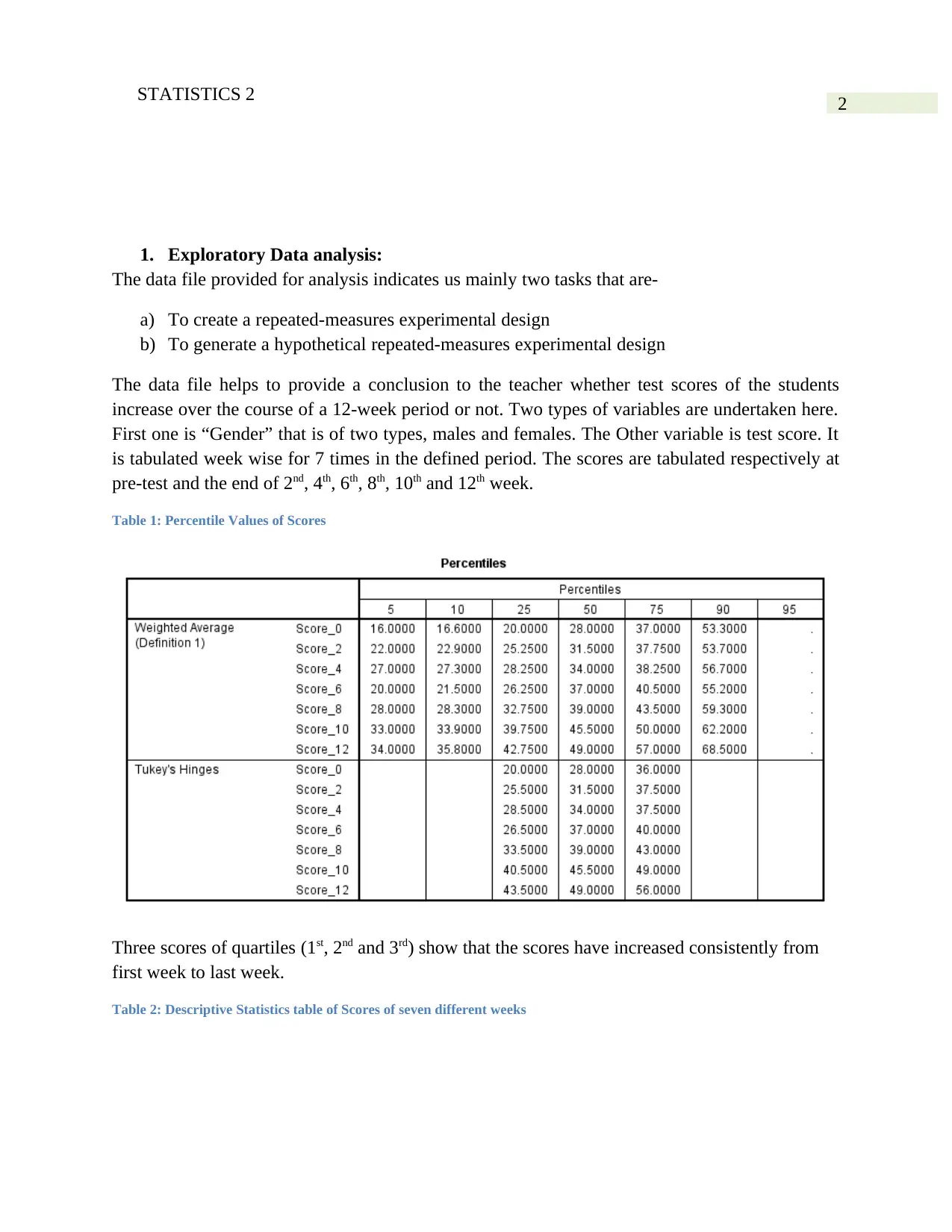
1. Exploratory Data analysis:
The data file provided for analysis indicates us mainly two tasks that are-
a) To create a repeated-measures experimental design
b) To generate a hypothetical repeated-measures experimental design
The data file helps to provide a conclusion to the teacher whether test scores of the students
increase over the course of a 12-week period or not. Two types of variables are undertaken here.
First one is “Gender” that is of two types, males and females. The Other variable is test score. It
is tabulated week wise for 7 times in the defined period. The scores are tabulated respectively at
pre-test and the end of 2nd, 4th, 6th, 8th, 10th and 12th week.
Table 1: Percentile Values of Scores
Three scores of quartiles (1st, 2nd and 3rd) show that the scores have increased consistently from
first week to last week.
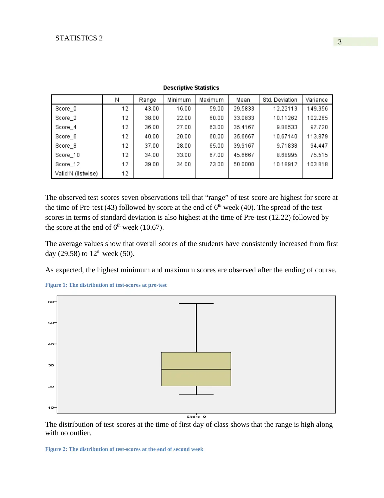
Table 2: Descriptive Statistics table of Scores of seven different weeks
1. Exploratory Data analysis:
The data file provided for analysis indicates us mainly two tasks that are-
a) To create a repeated-measures experimental design
b) To generate a hypothetical repeated-measures experimental design
The data file helps to provide a conclusion to the teacher whether test scores of the students
increase over the course of a 12-week period or not. Two types of variables are undertaken here.
First one is “Gender” that is of two types, males and females. The Other variable is test score. It
is tabulated week wise for 7 times in the defined period. The scores are tabulated respectively at
pre-test and the end of 2nd, 4th, 6th, 8th, 10th and 12th week.
Table 1: Percentile Values of Scores
Three scores of quartiles (1st, 2nd and 3rd) show that the scores have increased consistently from
first week to last week.
Table 2: Descriptive Statistics table of Scores of seven different weeks
3STATISTICS 2
The observed test-scores seven observations tell that “range” of test-score are highest for score at
the time of Pre-test (43) followed by score at the end of 6th week (40). The spread of the test-
scores in terms of standard deviation is also highest at the time of Pre-test (12.22) followed by
the score at the end of 6th week (10.67).
The average values show that overall scores of the students have consistently increased from first
day (29.58) to 12th week (50).
As expected, the highest minimum and maximum scores are observed after the ending of course.
Figure 1: The distribution of test-scores at pre-test
The distribution of test-scores at the time of first day of class shows that the range is high along
with no outlier.
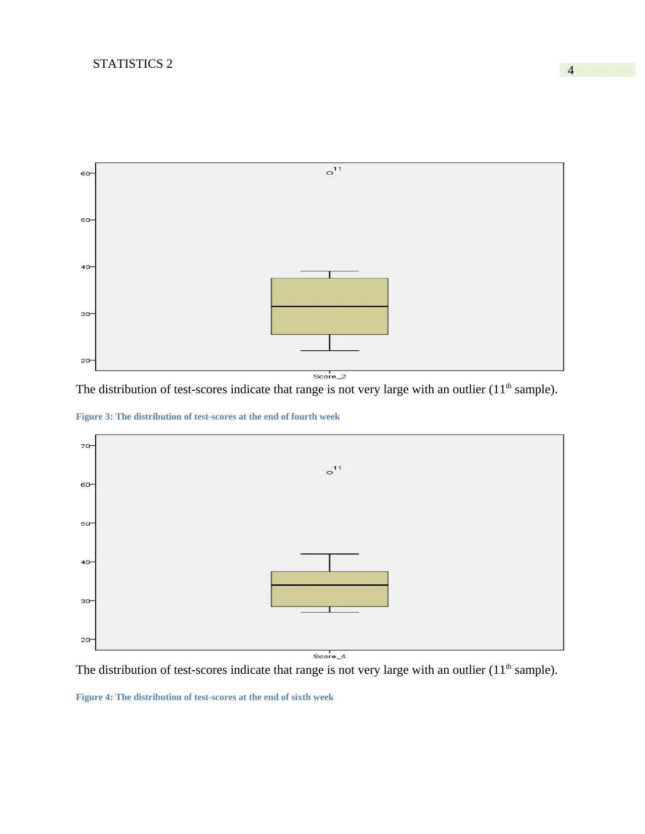
Figure 2: The distribution of test-scores at the end of second week
The observed test-scores seven observations tell that “range” of test-score are highest for score at
the time of Pre-test (43) followed by score at the end of 6th week (40). The spread of the test-
scores in terms of standard deviation is also highest at the time of Pre-test (12.22) followed by
the score at the end of 6th week (10.67).
The average values show that overall scores of the students have consistently increased from first
day (29.58) to 12th week (50).
As expected, the highest minimum and maximum scores are observed after the ending of course.
Figure 1: The distribution of test-scores at pre-test
The distribution of test-scores at the time of first day of class shows that the range is high along
with no outlier.
Figure 2: The distribution of test-scores at the end of second week
Secure Best Marks with AI Grader
Need help grading? Try our AI Grader for instant feedback on your assignments.
4STATISTICS 2
The distribution of test-scores indicate that range is not very large with an outlier (11th sample).
Figure 3: The distribution of test-scores at the end of fourth week
The distribution of test-scores indicate that range is not very large with an outlier (11th sample).
Figure 4: The distribution of test-scores at the end of sixth week
The distribution of test-scores indicate that range is not very large with an outlier (11th sample).
Figure 3: The distribution of test-scores at the end of fourth week
The distribution of test-scores indicate that range is not very large with an outlier (11th sample).
Figure 4: The distribution of test-scores at the end of sixth week
5STATISTICS 2
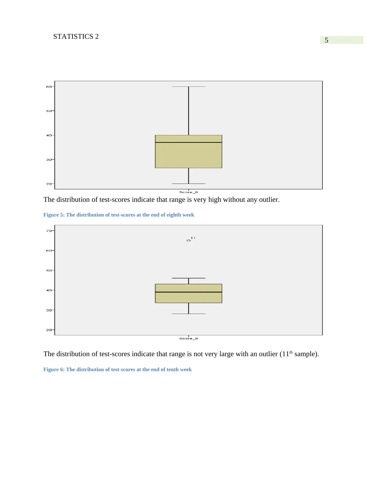
The distribution of test-scores indicate that range is very high without any outlier.
Figure 5: The distribution of test-scores at the end of eighth week
The distribution of test-scores indicate that range is not very large with an outlier (11th sample).
Figure 6: The distribution of test-scores at the end of tenth week
6STATISTICS 2
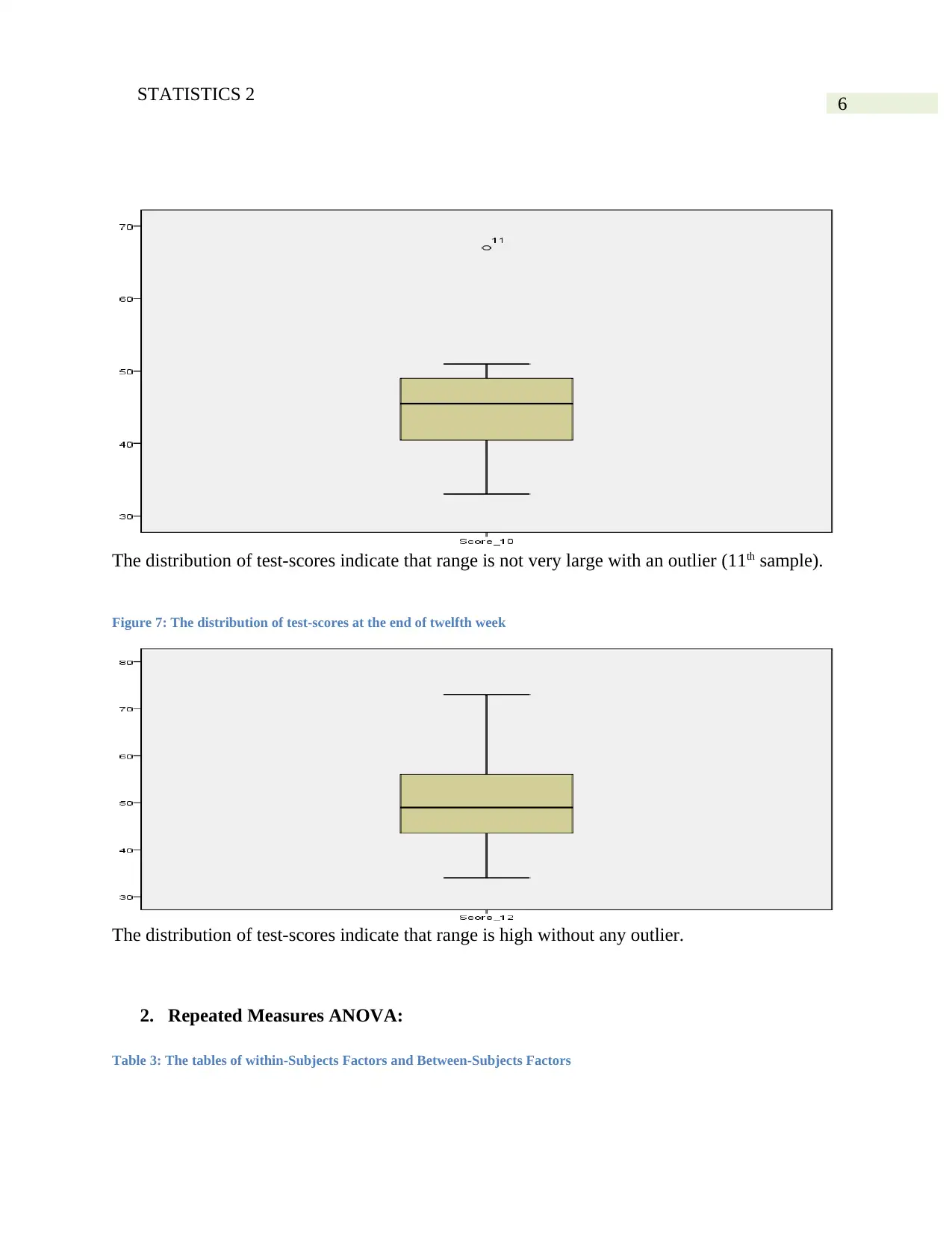
The distribution of test-scores indicate that range is not very large with an outlier (11th sample).
Figure 7: The distribution of test-scores at the end of twelfth week
The distribution of test-scores indicate that range is high without any outlier.
2. Repeated Measures ANOVA:
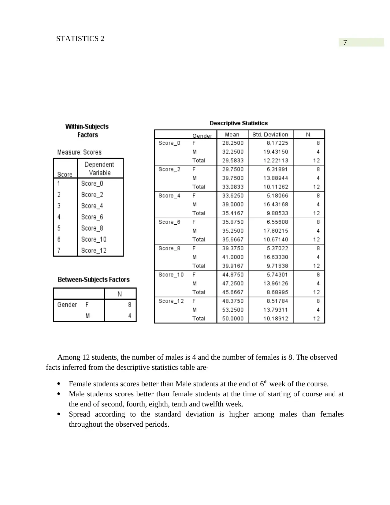
Table 3: The tables of within-Subjects Factors and Between-Subjects Factors
The distribution of test-scores indicate that range is not very large with an outlier (11th sample).
Figure 7: The distribution of test-scores at the end of twelfth week
The distribution of test-scores indicate that range is high without any outlier.
2. Repeated Measures ANOVA:
Table 3: The tables of within-Subjects Factors and Between-Subjects Factors
Paraphrase This Document
Need a fresh take? Get an instant paraphrase of this document with our AI Paraphraser
7STATISTICS 2
Among 12 students, the number of males is 4 and the number of females is 8. The observed
facts inferred from the descriptive statistics table are-
Female students scores better than Male students at the end of 6th week of the course.
Male students scores better than female students at the time of starting of course and at
the end of second, fourth, eighth, tenth and twelfth week.
Spread according to the standard deviation is higher among males than females
throughout the observed periods.
8STATISTICS 2
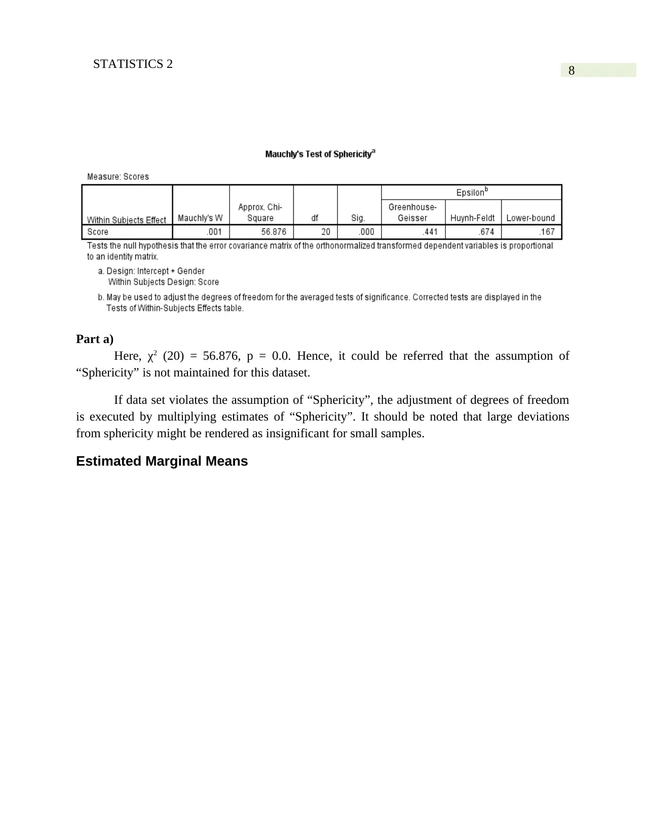
Part a)
Here, χ2 (20) = 56.876, p = 0.0. Hence, it could be referred that the assumption of
“Sphericity” is not maintained for this dataset.
If data set violates the assumption of “Sphericity”, the adjustment of degrees of freedom
is executed by multiplying estimates of “Sphericity”. It should be noted that large deviations
from sphericity might be rendered as insignificant for small samples.
Estimated Marginal Means
9STATISTICS 2
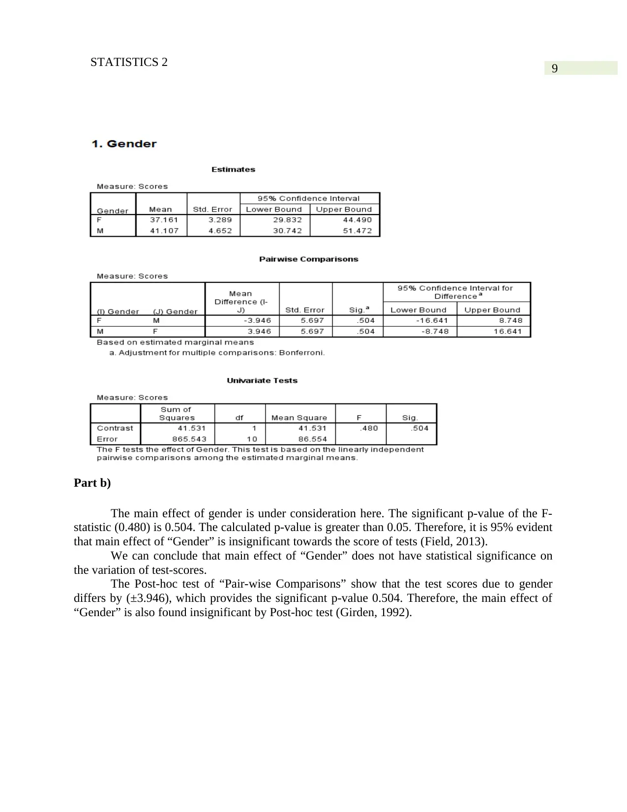
Part b)
The main effect of gender is under consideration here. The significant p-value of the F-
statistic (0.480) is 0.504. The calculated p-value is greater than 0.05. Therefore, it is 95% evident
that main effect of “Gender” is insignificant towards the score of tests (Field, 2013).
We can conclude that main effect of “Gender” does not have statistical significance on
the variation of test-scores.
The Post-hoc test of “Pair-wise Comparisons” show that the test scores due to gender
differs by (±3.946), which provides the significant p-value 0.504. Therefore, the main effect of
“Gender” is also found insignificant by Post-hoc test (Girden, 1992).
Secure Best Marks with AI Grader
Need help grading? Try our AI Grader for instant feedback on your assignments.
10STATISTICS 2
Pairwise Comparisons
Measure: Scores
(I) Score (J) Score Mean Difference
(I-J)
Std. Error Sig.b 95% Confidence Interval for
Differenceb
Lower Bound Upper Bound
1
2 -4.500 3.383 1.000 -18.151 9.151
3 -6.062 2.412 .645 -15.795 3.670
4 -5.312 2.117 .649 -13.853 3.228
5 -9.937 2.693 .088 -20.804 .929
6 -15.813* 2.683 .003 -26.638 -4.987
7 -20.563* 3.524 .003 -34.782 -6.343
2
1 4.500 3.383 1.000 -9.151 18.151
3 -1.562 1.542 1.000 -7.784 4.659
4 -.812 2.324 1.000 -10.188 8.563
5 -5.437 1.914 .368 -13.159 2.284
6 -11.313* 2.063 .006 -19.635 -2.990
7 -16.063* 3.154 .010 -28.787 -3.338
3 1 6.062 2.412 .645 -3.670 15.795
2 1.562 1.542 1.000 -4.659 7.784
4 .750 1.097 1.000 -3.674 5.174
5 -3.875 1.058 .092 -8.146 .396
11STATISTICS 2
6 -9.750* 1.336 .001 -15.139 -4.361
7 -14.500* 2.739 .007 -25.552 -3.448
4
1 5.312 2.117 .649 -3.228 13.853
2 .812 2.324 1.000 -8.563 10.188
3 -.750 1.097 1.000 -5.174 3.674
5 -4.625* 1.019 .023 -8.736 -.514
6 -10.500* 1.202 .000 -15.348 -5.652
7 -15.250* 2.711 .005 -26.189 -4.311
5
1 9.937 2.693 .088 -.929 20.804
2 5.437 1.914 .368 -2.284 13.159
3 3.875 1.058 .092 -.396 8.146
4 4.625* 1.019 .023 .514 8.736
6 -5.875* .716 .000 -8.766 -2.984
7 -10.625* 2.065 .009 -18.956 -2.294
6
1 15.813* 2.683 .003 4.987 26.638
2 11.313* 2.063 .006 2.990 19.635
3 9.750* 1.336 .001 4.361 15.139
4 10.500* 1.202 .000 5.652 15.348
5 5.875* .716 .000 2.984 8.766
7 -4.750 1.705 .404 -11.628 2.128
7
1 20.563* 3.524 .003 6.343 34.782
2 16.063* 3.154 .010 3.338 28.787
3 14.500* 2.739 .007 3.448 25.552
4 15.250* 2.711 .005 4.311 26.189
5 10.625* 2.065 .009 2.294 18.956
6 4.750 1.705 .404 -2.128 11.628
Based on estimated marginal means
*. The mean difference is significant at the .05 level.
b. Adjustment for multiple comparisons: Bonferroni.
12STATISTICS 2
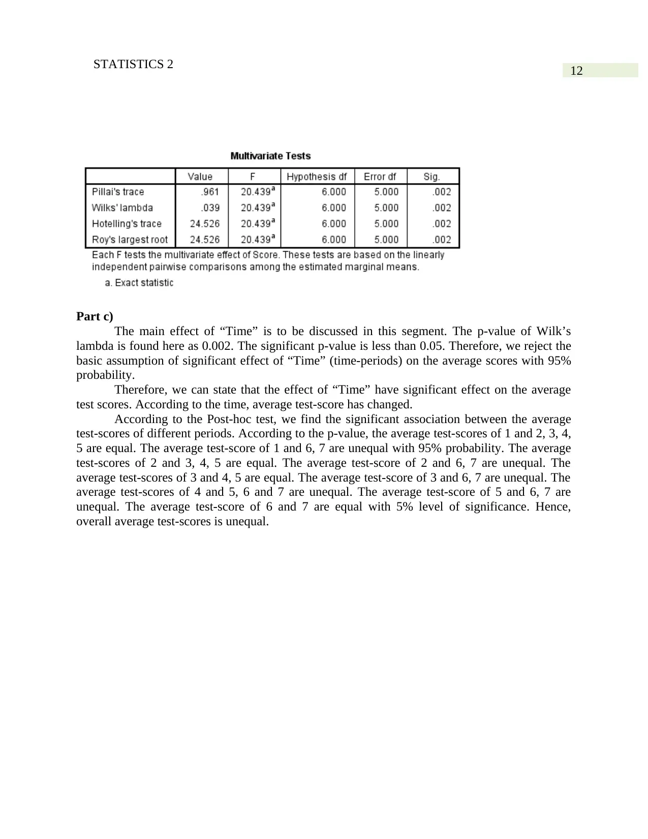
Part c)
The main effect of “Time” is to be discussed in this segment. The p-value of Wilk’s
lambda is found here as 0.002. The significant p-value is less than 0.05. Therefore, we reject the
basic assumption of significant effect of “Time” (time-periods) on the average scores with 95%
probability.
Therefore, we can state that the effect of “Time” have significant effect on the average
test scores. According to the time, average test-score has changed.
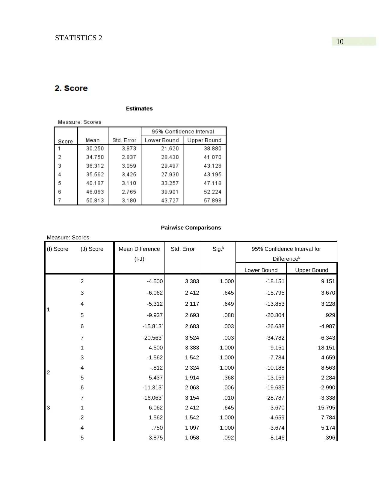
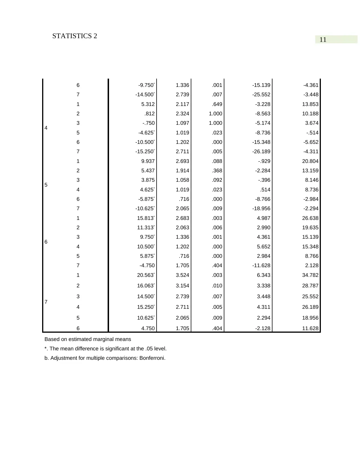
According to the Post-hoc test, we find the significant association between the average
test-scores of different periods. According to the p-value, the average test-scores of 1 and 2, 3, 4,
5 are equal. The average test-score of 1 and 6, 7 are unequal with 95% probability. The average
test-scores of 2 and 3, 4, 5 are equal. The average test-score of 2 and 6, 7 are unequal. The
average test-scores of 3 and 4, 5 are equal. The average test-score of 3 and 6, 7 are unequal. The
average test-scores of 4 and 5, 6 and 7 are unequal. The average test-score of 5 and 6, 7 are
unequal. The average test-score of 6 and 7 are equal with 5% level of significance. Hence,
overall average test-scores is unequal.
Part c)
The main effect of “Time” is to be discussed in this segment. The p-value of Wilk’s
lambda is found here as 0.002. The significant p-value is less than 0.05. Therefore, we reject the
basic assumption of significant effect of “Time” (time-periods) on the average scores with 95%
probability.
Therefore, we can state that the effect of “Time” have significant effect on the average
test scores. According to the time, average test-score has changed.
According to the Post-hoc test, we find the significant association between the average
test-scores of different periods. According to the p-value, the average test-scores of 1 and 2, 3, 4,
5 are equal. The average test-score of 1 and 6, 7 are unequal with 95% probability. The average
test-scores of 2 and 3, 4, 5 are equal. The average test-score of 2 and 6, 7 are unequal. The
average test-scores of 3 and 4, 5 are equal. The average test-score of 3 and 6, 7 are unequal. The
average test-scores of 4 and 5, 6 and 7 are unequal. The average test-score of 5 and 6, 7 are
unequal. The average test-score of 6 and 7 are equal with 5% level of significance. Hence,
overall average test-scores is unequal.
Paraphrase This Document
Need a fresh take? Get an instant paraphrase of this document with our AI Paraphraser
13STATISTICS 2
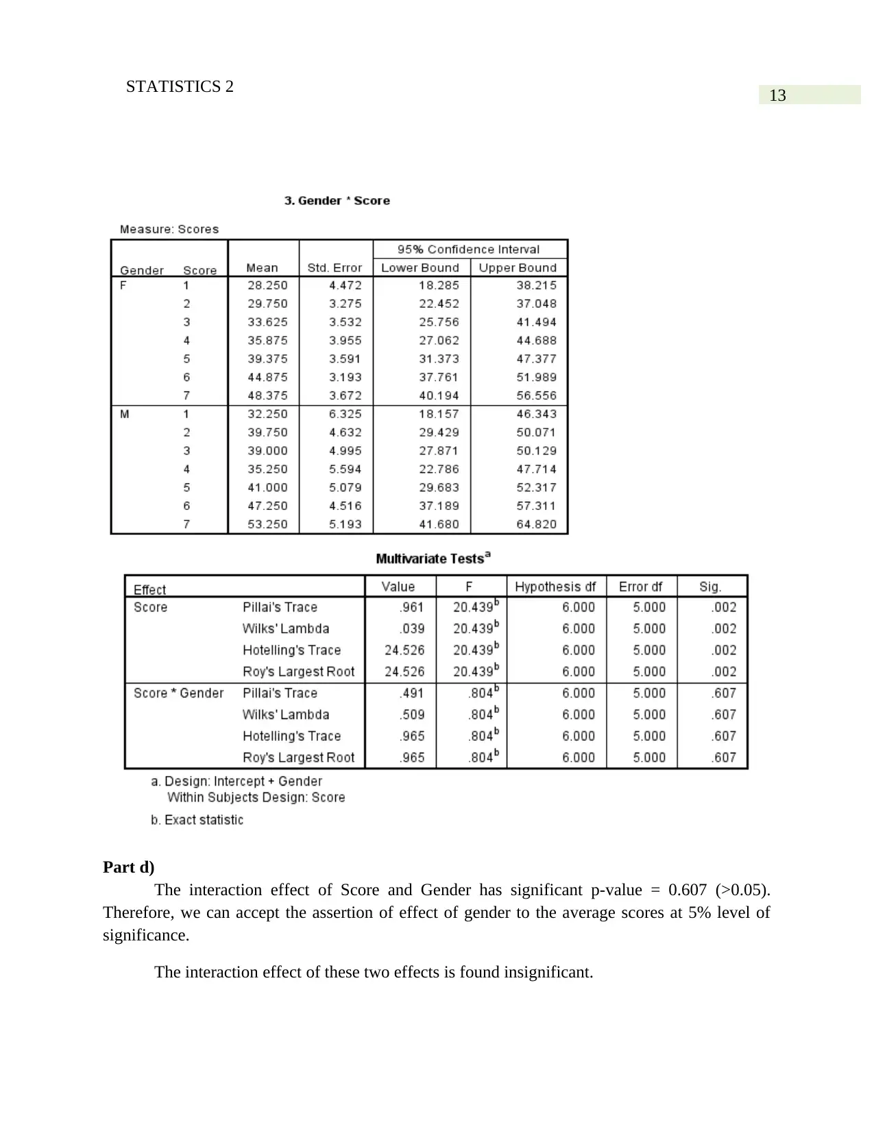
Part d)
The interaction effect of Score and Gender has significant p-value = 0.607 (>0.05).
Therefore, we can accept the assertion of effect of gender to the average scores at 5% level of
significance.
The interaction effect of these two effects is found insignificant.
Part d)
The interaction effect of Score and Gender has significant p-value = 0.607 (>0.05).
Therefore, we can accept the assertion of effect of gender to the average scores at 5% level of
significance.
The interaction effect of these two effects is found insignificant.
14STATISTICS 2
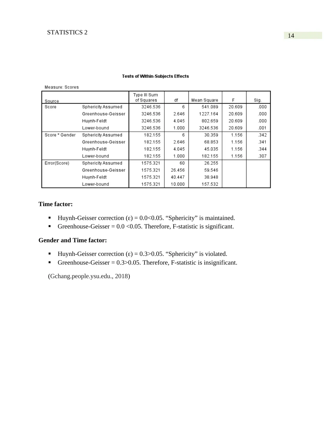
Time factor:
Huynh-Geisser correction (ε) = 0.0<0.05. “Sphericity” is maintained.
Greenhouse-Geisser = 0.0 <0.05. Therefore, F-statistic is significant.
Gender and Time factor:
Huynh-Geisser correction (ε) = 0.3>0.05. “Sphericity” is violated.
Greenhouse-Geisser = 0.3>0.05. Therefore, F-statistic is insignificant.
(Gchang.people.ysu.edu., 2018)
15STATISTICS 2
Secure Best Marks with AI Grader
Need help grading? Try our AI Grader for instant feedback on your assignments.
16STATISTICS 2
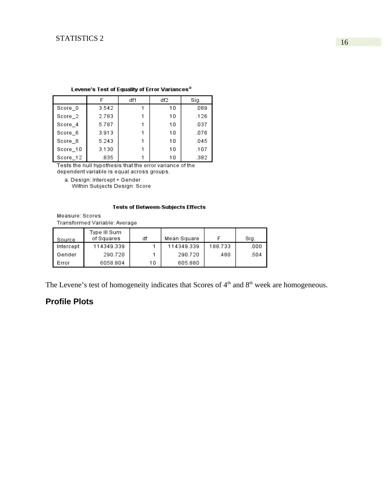
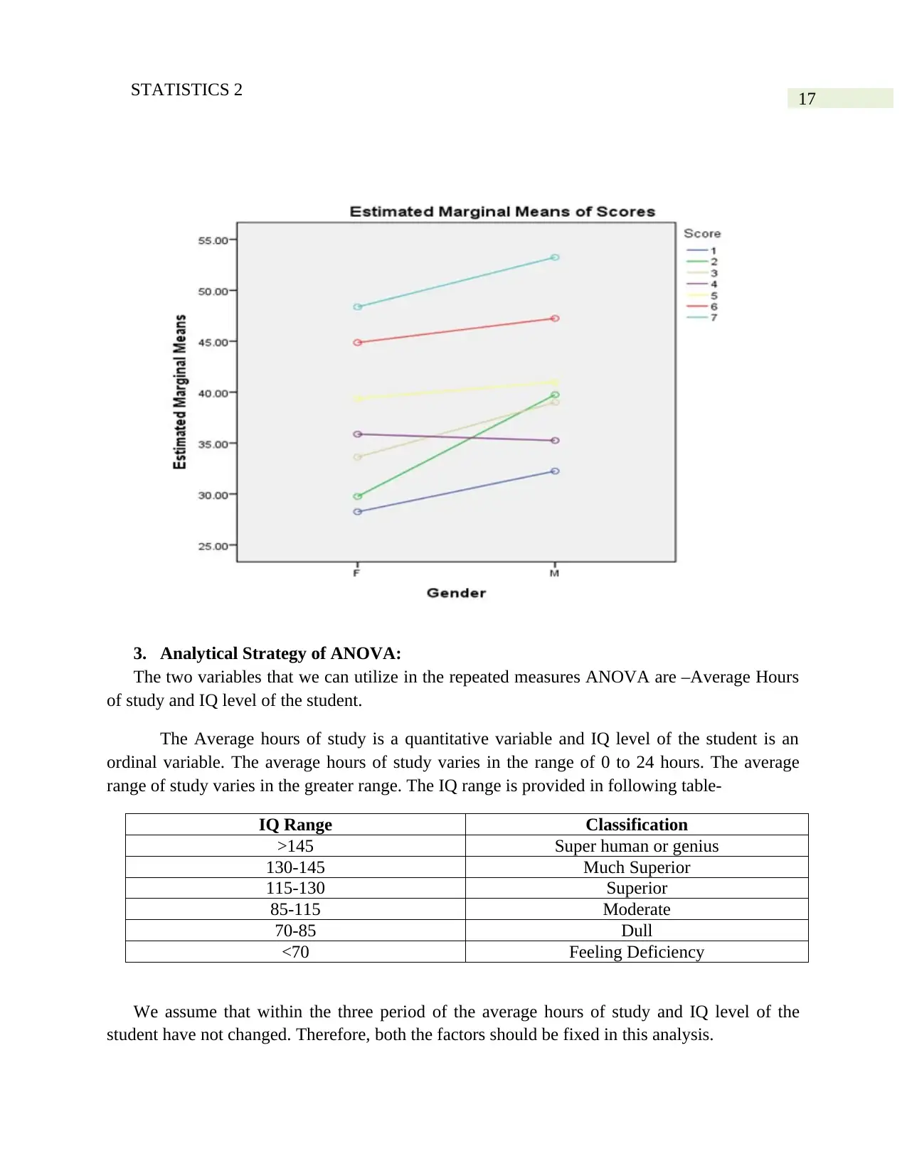
The Levene’s test of homogeneity indicates that Scores of 4th and 8th week are homogeneous.
Profile Plots
The Levene’s test of homogeneity indicates that Scores of 4th and 8th week are homogeneous.
Profile Plots
17STATISTICS 2
3. Analytical Strategy of ANOVA:
The two variables that we can utilize in the repeated measures ANOVA are –Average Hours
of study and IQ level of the student.
The Average hours of study is a quantitative variable and IQ level of the student is an
ordinal variable. The average hours of study varies in the range of 0 to 24 hours. The average
range of study varies in the greater range. The IQ range is provided in following table-
IQ Range Classification
>145 Super human or genius
130-145 Much Superior
115-130 Superior
85-115 Moderate
70-85 Dull
<70 Feeling Deficiency
We assume that within the three period of the average hours of study and IQ level of the
student have not changed. Therefore, both the factors should be fixed in this analysis.
18STATISTICS 2
In case of repeated measures ANOVA, the associations between pairs of experimental
conditions are alike. This assumption is called “Sphericity” (Health.uottawa.ca., 2018). It easily
cannot be compared to the tabulated values (ANOVA table) of the F-distribution. The significant
presence of violation of “Sphericity” could be found in-
1. Greenhouse and Geisser statistic
2. Huynh and Feldt statistic
3. The lower value estimate or the lowest possible theoretical value of the data
The “Greenhouse and Geisser statistic” and “Huynh and Feldt statistic” can both range from
the lower bound to 1. The Mauchly’s test examines whether the variances of the differences
between conditions are equal.
On the SPSS output, we look to find out Mauchly’s test statistic. If it has p-value less than
0.05, it could be concluded that there exists significant differences between variance of
differences as condition of “Sphericity” is violated.
The effect of violating “Sphericity” is actually losing the power of F-test in ANOVA. The
probability of type-II error gets increased in F-ratio. In that situation, adjustment of degrees of
freedom is necessary as it makes F-statistic more conservative. The smaller degrees of freedom
of Study hours, IQ level and their interaction effect would manage the issue of violation of
“Sphericity”.
Overall Thoughtful Consideration:
The repeated ANOVA calculation helps to draw conclusion that as the course time
proceeded, the average scores of tests overall increased. However, the effect of gender factor is
negligible in scores of different weeks. The performance in test is not varying significantly when
interaction effect of time and gender is considered. The addition of two chosen variable that are
average daily study hours and IQ level could provide a better analysis. However, it is mandatory
to be aware of maintaining “Sphericity” that previously was maintained in discussed analysis.
Otherwise, bias in conclusion may arise.
Paraphrase This Document
Need a fresh take? Get an instant paraphrase of this document with our AI Paraphraser
19STATISTICS 2
References:
Field, A. (2013). Discovering statistics using IBM SPSS statistics. sage.
Gchang.people.ysu.edu. (2018). Cite a Website - Cite This For Me. [online] Available at:
http://gchang.people.ysu.edu/SPSSE/SPSS_EDA_16.pdf.
Girden, E. R. (1992). ANOVA: Repeated measures (No. 84). Sage.
References:
Field, A. (2013). Discovering statistics using IBM SPSS statistics. sage.
Gchang.people.ysu.edu. (2018). Cite a Website - Cite This For Me. [online] Available at:
http://gchang.people.ysu.edu/SPSSE/SPSS_EDA_16.pdf.
Girden, E. R. (1992). ANOVA: Repeated measures (No. 84). Sage.
20STATISTICS 2
Health.uottawa.ca. (2018). Cite a Website - Cite This For Me. [online] Available at:
http://health.uottawa.ca/biomech/courses/apa6101/Repeated%20Measures%20ANOVA.pdf.
Health.uottawa.ca. (2018). Cite a Website - Cite This For Me. [online] Available at:
http://health.uottawa.ca/biomech/courses/apa6101/Repeated%20Measures%20ANOVA.pdf.
1 out of 21
Related Documents


Your All-in-One AI-Powered Toolkit for Academic Success.
+13062052269
info@desklib.com
Available 24*7 on WhatsApp / Email
![[object Object]](/_next/static/media/star-bottom.7253800d.svg)
Unlock your academic potential
© 2024 | Zucol Services PVT LTD | All rights reserved.