Digital Signal Processing PDF
VerifiedAdded on 2022/01/06
|15
|2551
|26
AI Summary
Contribute Materials
Your contribution can guide someone’s learning journey. Share your
documents today.

Digital Signal Processing
Student ID Number
Student Name
Student ID Number
Student Name
Secure Best Marks with AI Grader
Need help grading? Try our AI Grader for instant feedback on your assignments.
Part I (Filter design and signal analysis)
Problem 1
y [n]=1/21(−2 x[n]+3 x [n−1]+6 x [n−2]+7 x [ n−3 ]+6 x [n−4]+3 x [n−5 ]−2 x [n−6 ])Questio
n 1
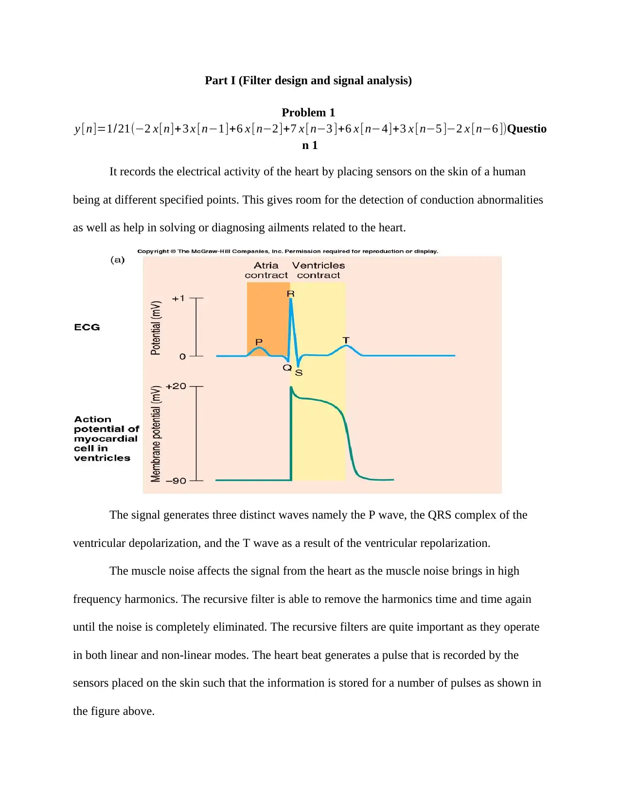
It records the electrical activity of the heart by placing sensors on the skin of a human
being at different specified points. This gives room for the detection of conduction abnormalities
as well as help in solving or diagnosing ailments related to the heart.
The signal generates three distinct waves namely the P wave, the QRS complex of the
ventricular depolarization, and the T wave as a result of the ventricular repolarization.
The muscle noise affects the signal from the heart as the muscle noise brings in high
frequency harmonics. The recursive filter is able to remove the harmonics time and time again
until the noise is completely eliminated. The recursive filters are quite important as they operate
in both linear and non-linear modes. The heart beat generates a pulse that is recorded by the
sensors placed on the skin such that the information is stored for a number of pulses as shown in
the figure above.
Problem 1
y [n]=1/21(−2 x[n]+3 x [n−1]+6 x [n−2]+7 x [ n−3 ]+6 x [n−4]+3 x [n−5 ]−2 x [n−6 ])Questio
n 1
It records the electrical activity of the heart by placing sensors on the skin of a human
being at different specified points. This gives room for the detection of conduction abnormalities
as well as help in solving or diagnosing ailments related to the heart.
The signal generates three distinct waves namely the P wave, the QRS complex of the
ventricular depolarization, and the T wave as a result of the ventricular repolarization.
The muscle noise affects the signal from the heart as the muscle noise brings in high
frequency harmonics. The recursive filter is able to remove the harmonics time and time again
until the noise is completely eliminated. The recursive filters are quite important as they operate
in both linear and non-linear modes. The heart beat generates a pulse that is recorded by the
sensors placed on the skin such that the information is stored for a number of pulses as shown in
the figure above.
It is important to process the signal recorded because it ensures that the harmonics are
eliminated and the doctors can easily analyze the signal to determine if the patient has a chronic
heart disease or not. The distorted signal may not provide the correct information as there are
disturbances that affect the signal and they are removed using the recursive filter.
Question 2
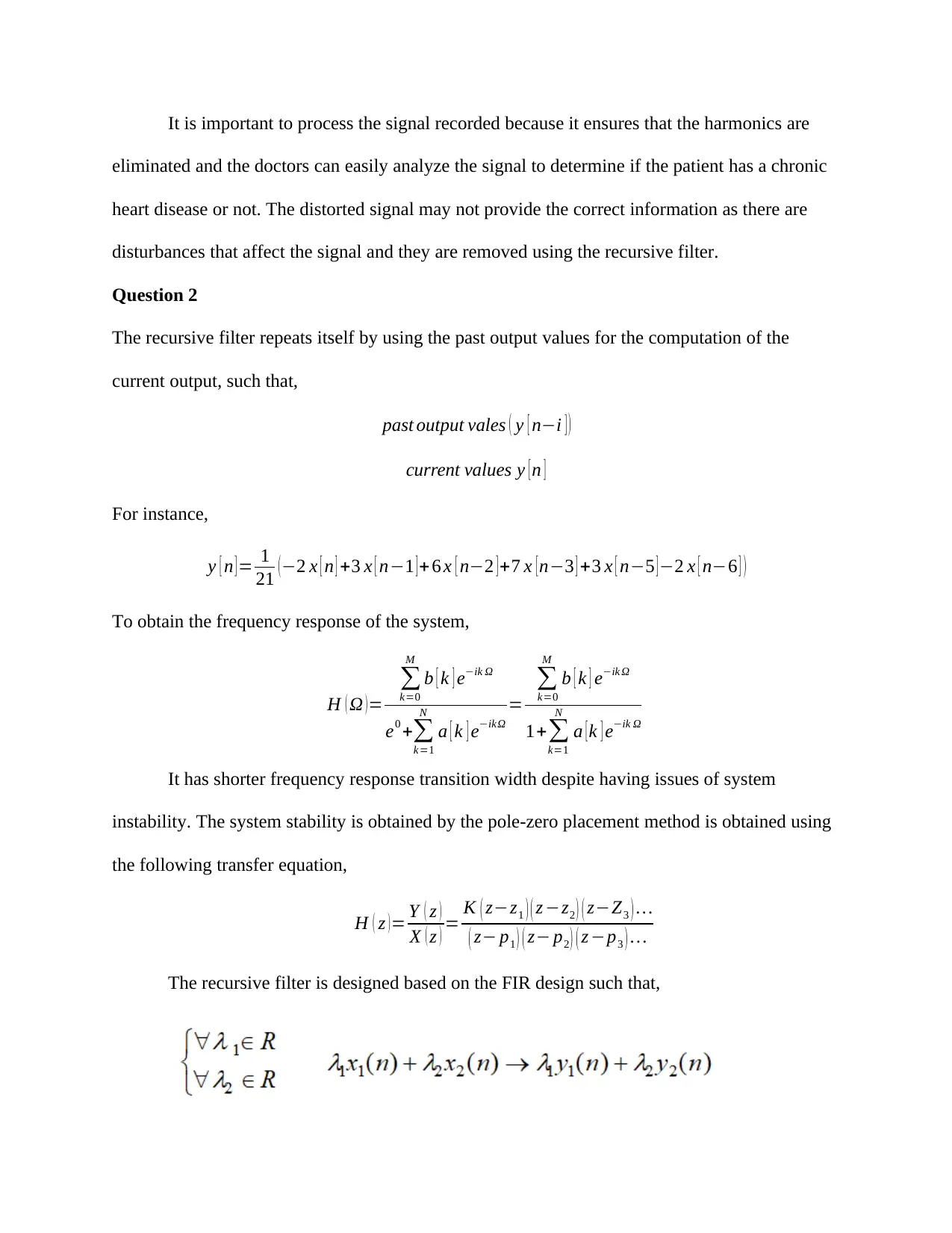
The recursive filter repeats itself by using the past output values for the computation of the
current output, such that,
past output vales ( y [ n−i ] )
current values y [ n ]
For instance,
y [ n ] = 1
21 (−2 x [ n ] +3 x [ n−1 ]+ 6 x [ n−2 ] +7 x [n−3 ] +3 x [ n−5 ]−2 x [ n−6 ] )
To obtain the frequency response of the system,
H ( Ω )=
∑
k=0
M
b [ k ] e−ik Ω
e0 +∑
k=1
N
a [ k ] e−ikΩ
=
∑
k=0
M
b [ k ] e−ik Ω
1+∑
k=1
N
a [ k ] e−ik Ω
It has shorter frequency response transition width despite having issues of system
instability. The system stability is obtained by the pole-zero placement method is obtained using
the following transfer equation,
H ( z ) = Y ( z )
X ( z ) = K ( z−z1 ) ( z −z2 ) ( z−Z3 ) …
( z− p1 ) ( z− p2 ) ( z −p3 ) …
The recursive filter is designed based on the FIR design such that,
eliminated and the doctors can easily analyze the signal to determine if the patient has a chronic
heart disease or not. The distorted signal may not provide the correct information as there are
disturbances that affect the signal and they are removed using the recursive filter.
Question 2
The recursive filter repeats itself by using the past output values for the computation of the
current output, such that,
past output vales ( y [ n−i ] )
current values y [ n ]
For instance,
y [ n ] = 1
21 (−2 x [ n ] +3 x [ n−1 ]+ 6 x [ n−2 ] +7 x [n−3 ] +3 x [ n−5 ]−2 x [ n−6 ] )
To obtain the frequency response of the system,
H ( Ω )=
∑
k=0
M
b [ k ] e−ik Ω
e0 +∑
k=1
N
a [ k ] e−ikΩ
=
∑
k=0
M
b [ k ] e−ik Ω
1+∑
k=1
N
a [ k ] e−ik Ω
It has shorter frequency response transition width despite having issues of system
instability. The system stability is obtained by the pole-zero placement method is obtained using
the following transfer equation,
H ( z ) = Y ( z )
X ( z ) = K ( z−z1 ) ( z −z2 ) ( z−Z3 ) …
( z− p1 ) ( z− p2 ) ( z −p3 ) …
The recursive filter is designed based on the FIR design such that,
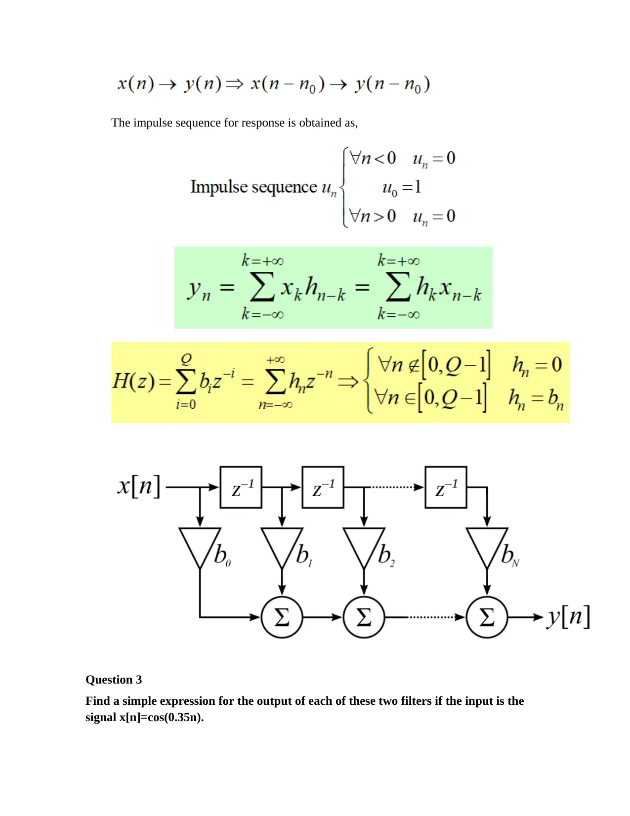
The impulse sequence for response is obtained as,
Question 3
Find a simple expression for the output of each of these two filters if the input is the
signal x[n]=cos(0.35n).
Question 3
Find a simple expression for the output of each of these two filters if the input is the
signal x[n]=cos(0.35n).
Secure Best Marks with AI Grader
Need help grading? Try our AI Grader for instant feedback on your assignments.
clear all
close all
clc
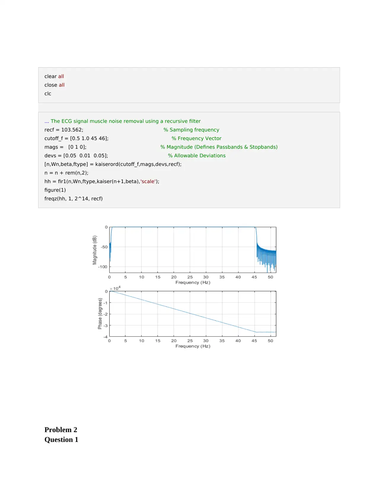
... The ECG signal muscle noise removal using a recursive filter
recf = 103.562; % Sampling frequency
cutoff_f = [0.5 1.0 45 46]; % Frequency Vector
mags = [0 1 0]; % Magnitude (Defines Passbands & Stopbands)
devs = [0.05 0.01 0.05]; % Allowable Deviations
[n,Wn,beta,ftype] = kaiserord(cutoff_f,mags,devs,recf);
n = n + rem(n,2);
hh = fir1(n,Wn,ftype,kaiser(n+1,beta),'scale');
figure(1)
freqz(hh, 1, 2^14, recf)
Problem 2
Question 1
close all
clc
... The ECG signal muscle noise removal using a recursive filter
recf = 103.562; % Sampling frequency
cutoff_f = [0.5 1.0 45 46]; % Frequency Vector
mags = [0 1 0]; % Magnitude (Defines Passbands & Stopbands)
devs = [0.05 0.01 0.05]; % Allowable Deviations
[n,Wn,beta,ftype] = kaiserord(cutoff_f,mags,devs,recf);
n = n + rem(n,2);
hh = fir1(n,Wn,ftype,kaiser(n+1,beta),'scale');
figure(1)
freqz(hh, 1, 2^14, recf)
Problem 2
Question 1
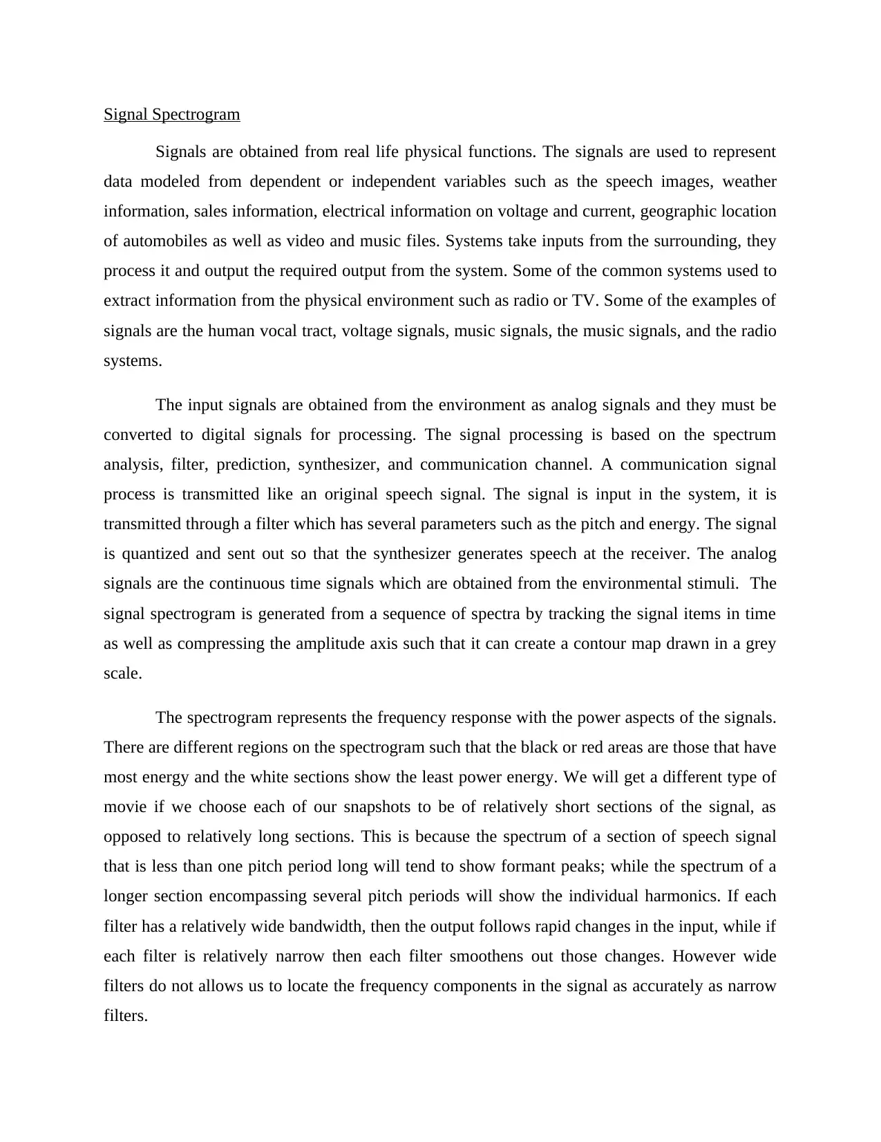
Signal Spectrogram
Signals are obtained from real life physical functions. The signals are used to represent
data modeled from dependent or independent variables such as the speech images, weather
information, sales information, electrical information on voltage and current, geographic location
of automobiles as well as video and music files. Systems take inputs from the surrounding, they
process it and output the required output from the system. Some of the common systems used to
extract information from the physical environment such as radio or TV. Some of the examples of
signals are the human vocal tract, voltage signals, music signals, the music signals, and the radio
systems.
The input signals are obtained from the environment as analog signals and they must be
converted to digital signals for processing. The signal processing is based on the spectrum
analysis, filter, prediction, synthesizer, and communication channel. A communication signal
process is transmitted like an original speech signal. The signal is input in the system, it is
transmitted through a filter which has several parameters such as the pitch and energy. The signal
is quantized and sent out so that the synthesizer generates speech at the receiver. The analog
signals are the continuous time signals which are obtained from the environmental stimuli. The
signal spectrogram is generated from a sequence of spectra by tracking the signal items in time
as well as compressing the amplitude axis such that it can create a contour map drawn in a grey
scale.
The spectrogram represents the frequency response with the power aspects of the signals.
There are different regions on the spectrogram such that the black or red areas are those that have
most energy and the white sections show the least power energy. We will get a different type of
movie if we choose each of our snapshots to be of relatively short sections of the signal, as
opposed to relatively long sections. This is because the spectrum of a section of speech signal
that is less than one pitch period long will tend to show formant peaks; while the spectrum of a
longer section encompassing several pitch periods will show the individual harmonics. If each
filter has a relatively wide bandwidth, then the output follows rapid changes in the input, while if
each filter is relatively narrow then each filter smoothens out those changes. However wide
filters do not allows us to locate the frequency components in the signal as accurately as narrow
filters.
For a short time Fourier transform, a signal is obtained from the fast Fourier transform
which converts the signal from the continuous time based on a window sliding with time. The
spectrogram is the evolution of the magnitude with time. The windowing space has some effects
such as the main lobe and the side lobes. The window length determines the side of the
frequency resolution with m depending on the window. There are different types of windows
such as the rectangular, hamming, and Blackman. It determines a good resolution in time or in
frequency, or not in both. It provides good localization in time and the frequency. To convert the
signal from the continuous time signal to digital time signal, a sampling rate is determined on
periodic basis. The remains from the sampling are the values of the analog signal at discrete time
points hence it is a discrete time signals. The signal digitization represented based on the nyquist
theorem. When lower sampling rates are used, the bandwidth or storage is saved and
computation speeds up.
It is required that once the signal is sampled, it must be passed through a low pass filter
and it may avoid distortions from the aliasing. The sampled value is digitized and the analog
inputs are set at fixed discrete levels and mapped to the nearest discrete levels. The digitization
of the signals may be a linear or a non-linear process based on the signal uniformity. The features
of a signal need to be captured under the spectral attributes of the signal. It is crucial to
determine the salient spectral attributes of the sound signal. The information operates on the
speaker-specific or any other incidental structures. The signal spectrogram is computed and a set
of numbers are used to capture only salient aspects of the spectrogram. The discrete Fourier
transform has components of the time series that are complex exponentials whose analysis
determines the weights of the component time series. A DFT transform decomposes the signal
into a collection of finite number of complex exponentials. There are many exponentials that are
sampled in the signal being analyzed. The function computes the Fourier spectrum of a periodic
signal on infinite limits.
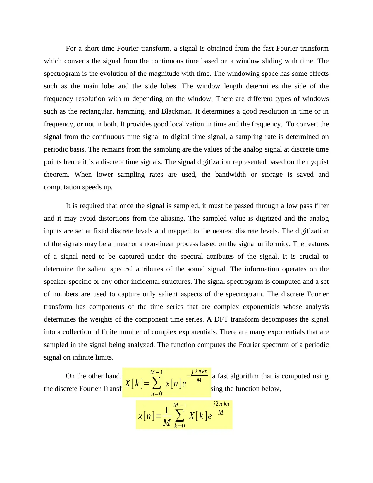
On the other hand the Fast Fourier Transform is a fast algorithm that is computed using
the discrete Fourier Transform. The signal is recovered using the function below,
X [ k ]= ∑
n=0
M −1
x [n ]e− j 2 π kn
M
x [n ]= 1
M ∑
k =0
M −1
X [ k ]e
j2 π kn
M
which converts the signal from the continuous time based on a window sliding with time. The
spectrogram is the evolution of the magnitude with time. The windowing space has some effects
such as the main lobe and the side lobes. The window length determines the side of the
frequency resolution with m depending on the window. There are different types of windows
such as the rectangular, hamming, and Blackman. It determines a good resolution in time or in
frequency, or not in both. It provides good localization in time and the frequency. To convert the
signal from the continuous time signal to digital time signal, a sampling rate is determined on
periodic basis. The remains from the sampling are the values of the analog signal at discrete time
points hence it is a discrete time signals. The signal digitization represented based on the nyquist
theorem. When lower sampling rates are used, the bandwidth or storage is saved and
computation speeds up.
It is required that once the signal is sampled, it must be passed through a low pass filter
and it may avoid distortions from the aliasing. The sampled value is digitized and the analog
inputs are set at fixed discrete levels and mapped to the nearest discrete levels. The digitization
of the signals may be a linear or a non-linear process based on the signal uniformity. The features
of a signal need to be captured under the spectral attributes of the signal. It is crucial to
determine the salient spectral attributes of the sound signal. The information operates on the
speaker-specific or any other incidental structures. The signal spectrogram is computed and a set
of numbers are used to capture only salient aspects of the spectrogram. The discrete Fourier
transform has components of the time series that are complex exponentials whose analysis
determines the weights of the component time series. A DFT transform decomposes the signal
into a collection of finite number of complex exponentials. There are many exponentials that are
sampled in the signal being analyzed. The function computes the Fourier spectrum of a periodic
signal on infinite limits.
On the other hand the Fast Fourier Transform is a fast algorithm that is computed using
the discrete Fourier Transform. The signal is recovered using the function below,
X [ k ]= ∑
n=0
M −1
x [n ]e− j 2 π kn
M
x [n ]= 1
M ∑
k =0
M −1
X [ k ]e
j2 π kn
M
Paraphrase This Document
Need a fresh take? Get an instant paraphrase of this document with our AI Paraphraser
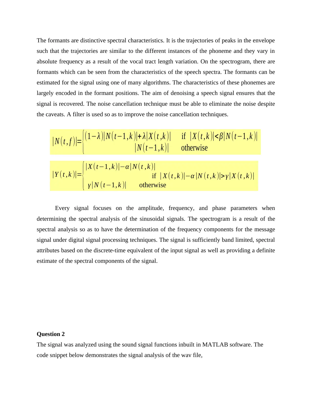
The formants are distinctive spectral characteristics. It is the trajectories of peaks in the envelope
such that the trajectories are similar to the different instances of the phoneme and they vary in
absolute frequency as a result of the vocal tract length variation. On the spectrogram, there are
formants which can be seen from the characteristics of the speech spectra. The formants can be
estimated for the signal using one of many algorithms. The characteristics of these phonemes are
largely encoded in the formant positions. The aim of denoising a speech signal ensures that the
signal is recovered. The noise cancellation technique must be able to eliminate the noise despite
the caveats. A filter is used so as to improve the noise cancellation techniques.
Every signal focuses on the amplitude, frequency, and phase parameters when
determining the spectral analysis of the sinusoidal signals. The spectrogram is a result of the
spectral analysis so as to have the determination of the frequency components for the message
signal under digital signal processing techniques. The signal is sufficiently band limited, spectral
attributes based on the discrete-time equivalent of the input signal as well as providing a definite
estimate of the spectral components of the signal.
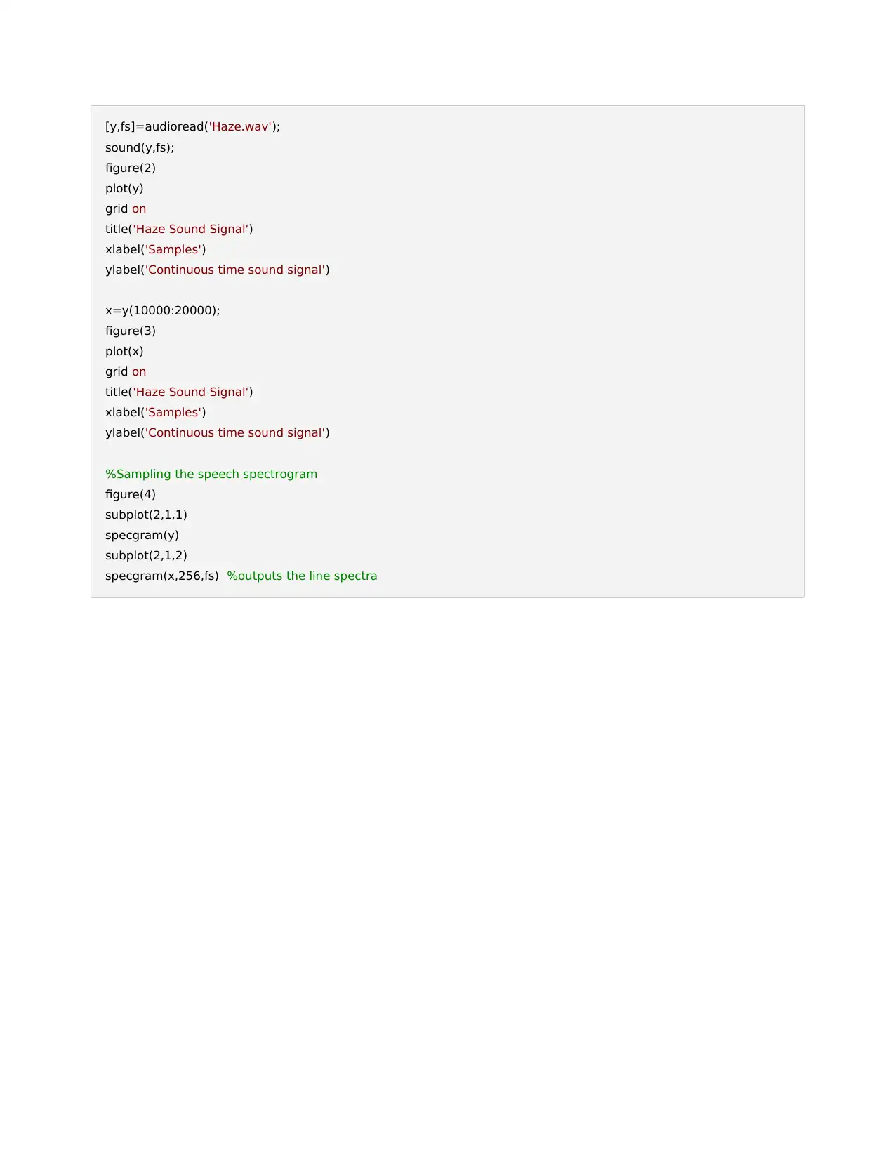
Question 2
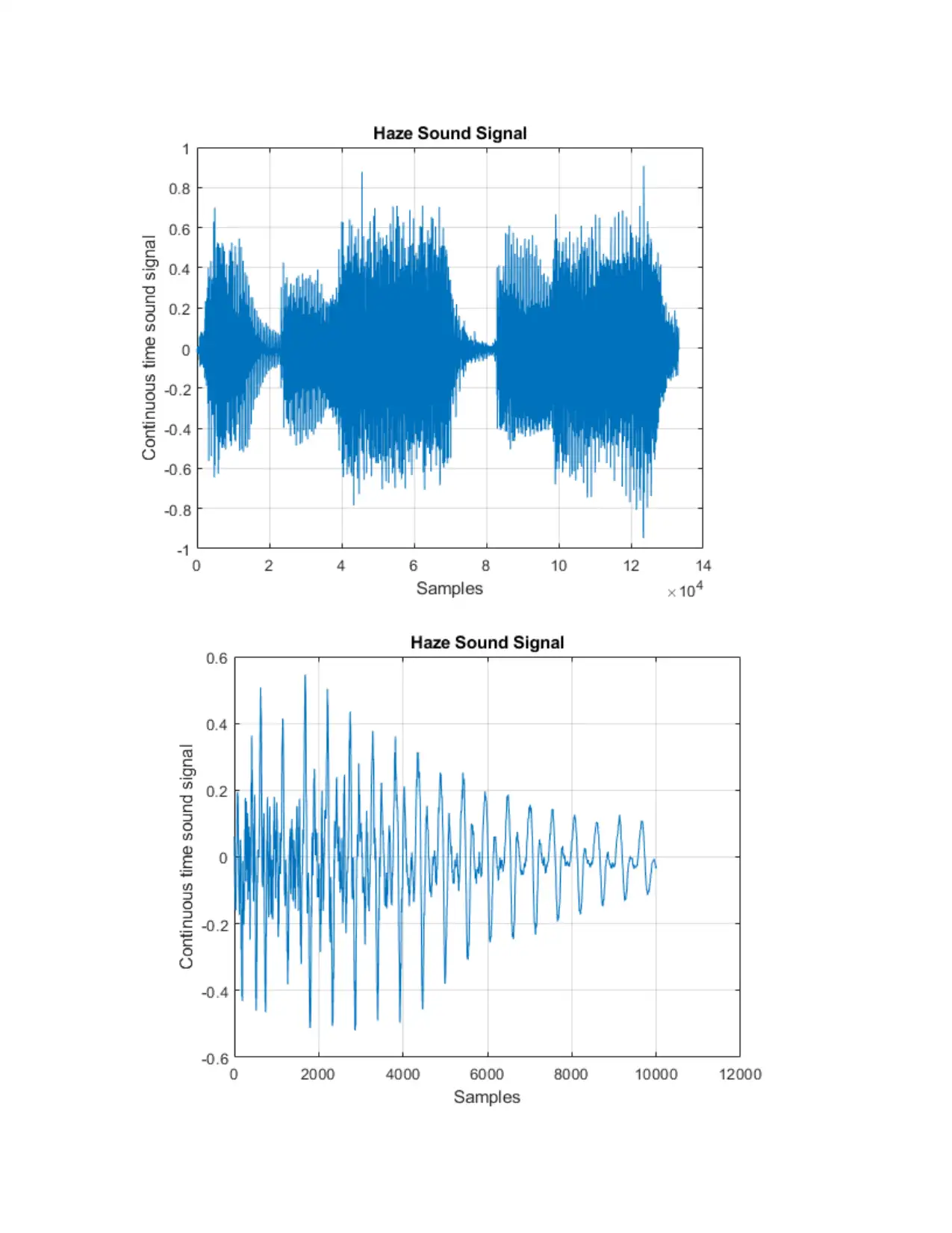
The signal was analyzed using the sound signal functions inbuilt in MATLAB software. The
code snippet below demonstrates the signal analysis of the wav file,
|N (t , f )|= {(1−λ )|N (t−1 , k )|+ λ|X (t ,k )| if |X (t , k )|< β|N (t −1 , k )|
|N (t −1 , k )| otherwise
|Y (t , k )|= {
|X (t−1 , k )|−α|N (t , k )|
if | X (t , k )|−α |N (t , k )|> γ|X (t , k )|
γ|N (t −1, k )| otherwise
such that the trajectories are similar to the different instances of the phoneme and they vary in
absolute frequency as a result of the vocal tract length variation. On the spectrogram, there are
formants which can be seen from the characteristics of the speech spectra. The formants can be
estimated for the signal using one of many algorithms. The characteristics of these phonemes are
largely encoded in the formant positions. The aim of denoising a speech signal ensures that the
signal is recovered. The noise cancellation technique must be able to eliminate the noise despite
the caveats. A filter is used so as to improve the noise cancellation techniques.
Every signal focuses on the amplitude, frequency, and phase parameters when
determining the spectral analysis of the sinusoidal signals. The spectrogram is a result of the
spectral analysis so as to have the determination of the frequency components for the message
signal under digital signal processing techniques. The signal is sufficiently band limited, spectral
attributes based on the discrete-time equivalent of the input signal as well as providing a definite
estimate of the spectral components of the signal.
Question 2
The signal was analyzed using the sound signal functions inbuilt in MATLAB software. The
code snippet below demonstrates the signal analysis of the wav file,
|N (t , f )|= {(1−λ )|N (t−1 , k )|+ λ|X (t ,k )| if |X (t , k )|< β|N (t −1 , k )|
|N (t −1 , k )| otherwise
|Y (t , k )|= {
|X (t−1 , k )|−α|N (t , k )|
if | X (t , k )|−α |N (t , k )|> γ|X (t , k )|
γ|N (t −1, k )| otherwise
[y,fs]=audioread('Haze.wav');
sound(y,fs);
figure(2)
plot(y)
grid on
title('Haze Sound Signal')
xlabel('Samples')
ylabel('Continuous time sound signal')
x=y(10000:20000);
figure(3)
plot(x)
grid on
title('Haze Sound Signal')
xlabel('Samples')
ylabel('Continuous time sound signal')
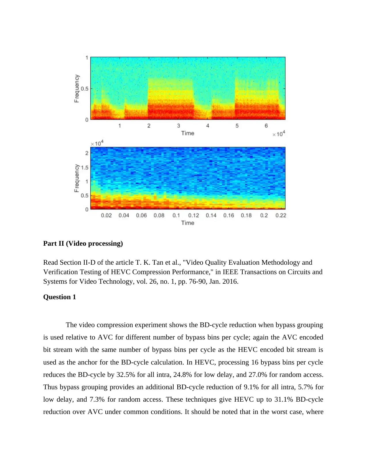
%Sampling the speech spectrogram
figure(4)
subplot(2,1,1)
specgram(y)
subplot(2,1,2)
specgram(x,256,fs) %outputs the line spectra
sound(y,fs);
figure(2)
plot(y)
grid on
title('Haze Sound Signal')
xlabel('Samples')
ylabel('Continuous time sound signal')
x=y(10000:20000);
figure(3)
plot(x)
grid on
title('Haze Sound Signal')
xlabel('Samples')
ylabel('Continuous time sound signal')
%Sampling the speech spectrogram
figure(4)
subplot(2,1,1)
specgram(y)
subplot(2,1,2)
specgram(x,256,fs) %outputs the line spectra
Secure Best Marks with AI Grader
Need help grading? Try our AI Grader for instant feedback on your assignments.
Part II (Video processing)
Read Section II-D of the article T. K. Tan et al., "Video Quality Evaluation Methodology and
Verification Testing of HEVC Compression Performance," in IEEE Transactions on Circuits and
Systems for Video Technology, vol. 26, no. 1, pp. 76-90, Jan. 2016.
Question 1
The video compression experiment shows the BD-cycle reduction when bypass grouping
is used relative to AVC for different number of bypass bins per cycle; again the AVC encoded
bit stream with the same number of bypass bins per cycle as the HEVC encoded bit stream is
used as the anchor for the BD-cycle calculation. In HEVC, processing 16 bypass bins per cycle
reduces the BD-cycle by 32.5% for all intra, 24.8% for low delay, and 27.0% for random access.
Thus bypass grouping provides an additional BD-cycle reduction of 9.1% for all intra, 5.7% for
low delay, and 7.3% for random access. These techniques give HEVC up to 31.1% BD-cycle
reduction over AVC under common conditions. It should be noted that in the worst case, where
bypass bins account for over 90 per cent of the total bins, cycle reduction of up to50 per cent is
achieved [6].
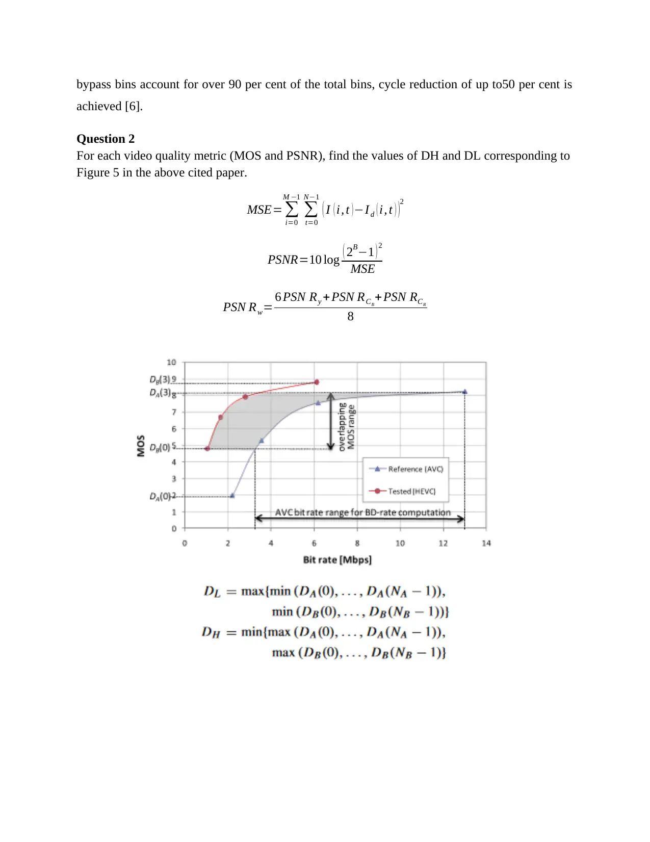
Question 2
For each video quality metric (MOS and PSNR), find the values of DH and DL corresponding to
Figure 5 in the above cited paper.
MSE= ∑
i=0
M −1
∑
t=0
N−1
( I ( i, t )−I d ( i, t ) )2
PSNR=10 log ( 2B−1 ) 2
MSE
PSN Rw= 6 PSN Ry + PSN RCB
+ PSN RCR
8
achieved [6].
Question 2
For each video quality metric (MOS and PSNR), find the values of DH and DL corresponding to
Figure 5 in the above cited paper.
MSE= ∑
i=0
M −1
∑
t=0
N−1
( I ( i, t )−I d ( i, t ) )2
PSNR=10 log ( 2B−1 ) 2
MSE
PSN Rw= 6 PSN Ry + PSN RCB
+ PSN RCR
8
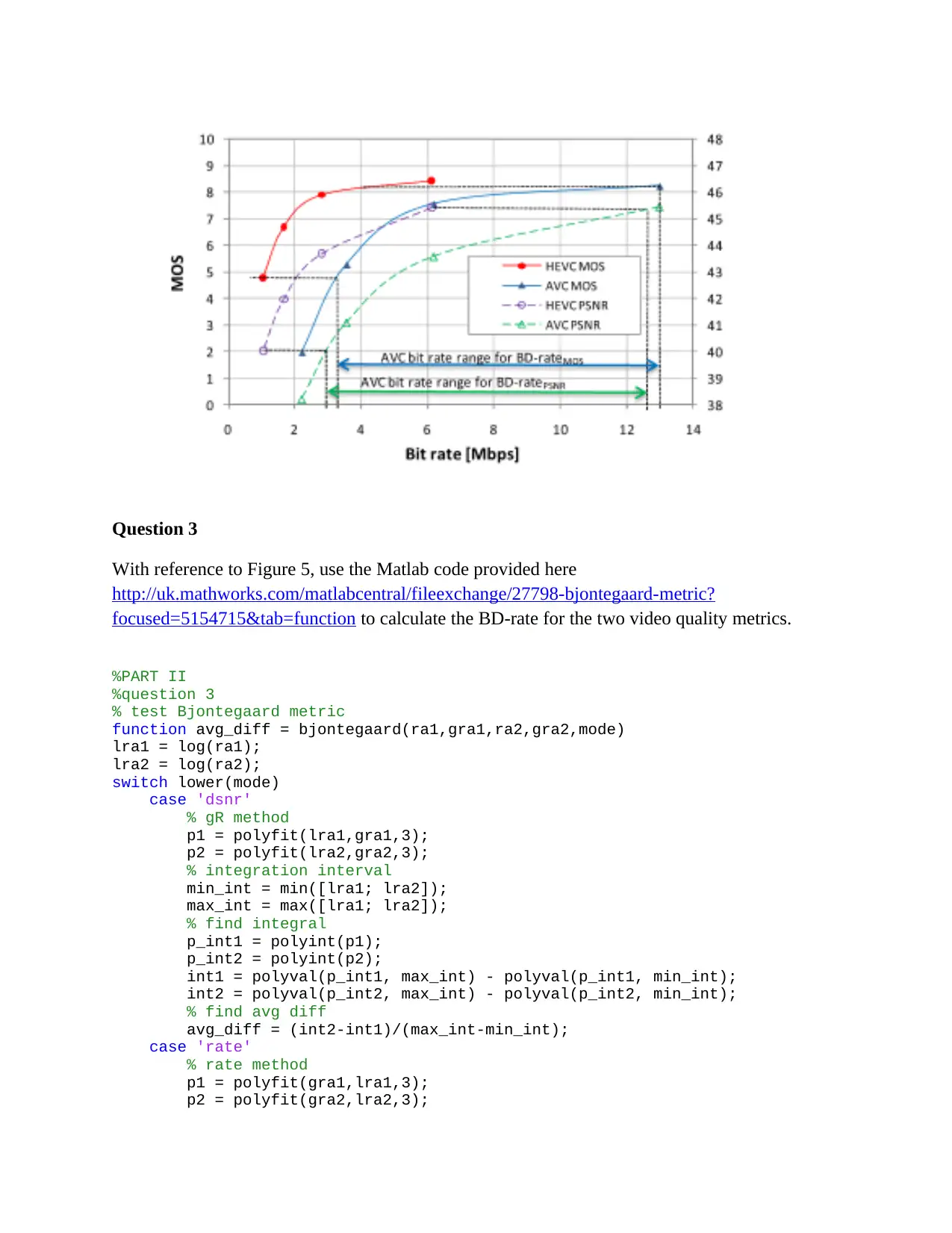
Question 3
With reference to Figure 5, use the Matlab code provided here
http://uk.mathworks.com/matlabcentral/fileexchange/27798-bjontegaard-metric?
focused=5154715&tab=function to calculate the BD-rate for the two video quality metrics.
%PART II
%question 3
% test Bjontegaard metric
function avg_diff = bjontegaard(ra1,gra1,ra2,gra2,mode)
lra1 = log(ra1);
lra2 = log(ra2);
switch lower(mode)
case 'dsnr'
% gR method
p1 = polyfit(lra1,gra1,3);
p2 = polyfit(lra2,gra2,3);
% integration interval
min_int = min([lra1; lra2]);
max_int = max([lra1; lra2]);
% find integral
p_int1 = polyint(p1);
p_int2 = polyint(p2);
int1 = polyval(p_int1, max_int) - polyval(p_int1, min_int);
int2 = polyval(p_int2, max_int) - polyval(p_int2, min_int);
% find avg diff
avg_diff = (int2-int1)/(max_int-min_int);
case 'rate'
% rate method
p1 = polyfit(gra1,lra1,3);
p2 = polyfit(gra2,lra2,3);
Paraphrase This Document
Need a fresh take? Get an instant paraphrase of this document with our AI Paraphraser
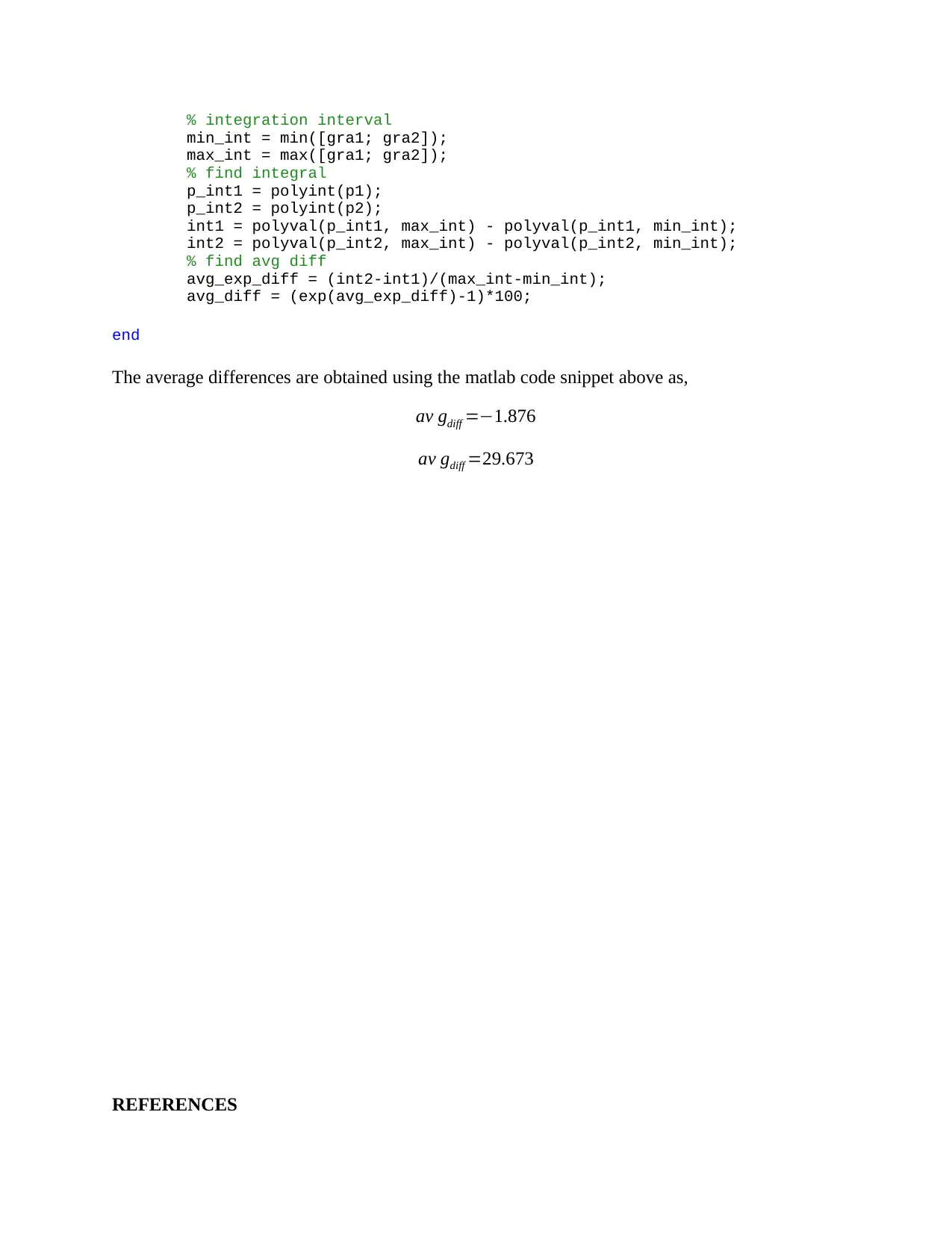
% integration interval
min_int = min([gra1; gra2]);
max_int = max([gra1; gra2]);
% find integral
p_int1 = polyint(p1);
p_int2 = polyint(p2);
int1 = polyval(p_int1, max_int) - polyval(p_int1, min_int);
int2 = polyval(p_int2, max_int) - polyval(p_int2, min_int);
% find avg diff
avg_exp_diff = (int2-int1)/(max_int-min_int);
avg_diff = (exp(avg_exp_diff)-1)*100;
end
The average differences are obtained using the matlab code snippet above as,
av gdiff =−1.876
av gdiff =29.673
REFERENCES
[1]. P. Artameeyanant. Image watermarking using adaptive tabu search. In ICCAS-SICE,
2009, pages 1941 –1944, aug. 2009.
[2]. Lijie Liu and Guoliang Fan. A new jpeg2000 region-of-interest image coding method:
partial significant bit planes shift. Signal Processing Letters, IEEE, 10(2):35 – 38, feb
2003.
[3]. Strang G. and Strela V., “Short Wavelets and Matrix Dilation Equations,” IEEE
Transactions Signal Processing, vol. 43, pp. 108-115, 2005.
[4]. Vetterli M. and Kovacevic J., Wavelets and Sub band Coding, Englewood Cliffs,
Prentice Hall, 1995, http /cm.bell-labs.com/ who/ jelena/Book/ home.html.
[5]. Wiegand T., Sullivan G., Bjontegaard G., and Luthra A., “Overview of the H.264 / AVC
Video Coding Standard,” IEEE Transactions on Circuits System Video Technology, pp.
243-250, 2003.
[6]. Wonkookim and Chung C., “On Preconditioning Multi wavelet System for Image
Compression,” International Journal of Wavelets Multi resolution and Information
Processing, vol. 1, no. 1, pp. 51-74, 2003.
[7]. K. R. Namuduri and V. N. Ramaswamy, “Feature preserving image compression,” in
Pattern Recognition Letters, vol. 24, no. 15, pp. 2767-2776, Nov. 2003.
1 out of 15


Your All-in-One AI-Powered Toolkit for Academic Success.
+13062052269
info@desklib.com
Available 24*7 on WhatsApp / Email
![[object Object]](/_next/static/media/star-bottom.7253800d.svg)
Unlock your academic potential
© 2024 | Zucol Services PVT LTD | All rights reserved.