Econometrics: Joint Probability Distribution, Marginal Probability Distribution, Expected Value, Variance, Covariance, Conditional Distribution, Population Regression Line

This document discusses various topics in econometrics including joint probability distribution, marginal probability distribution, expected value, variance, covariance, conditional distribution, and population regression line.

Running head: Econometrics
Econometrics
Name of the student
Name of the university
Course name
Course ID:

1
Econometrics
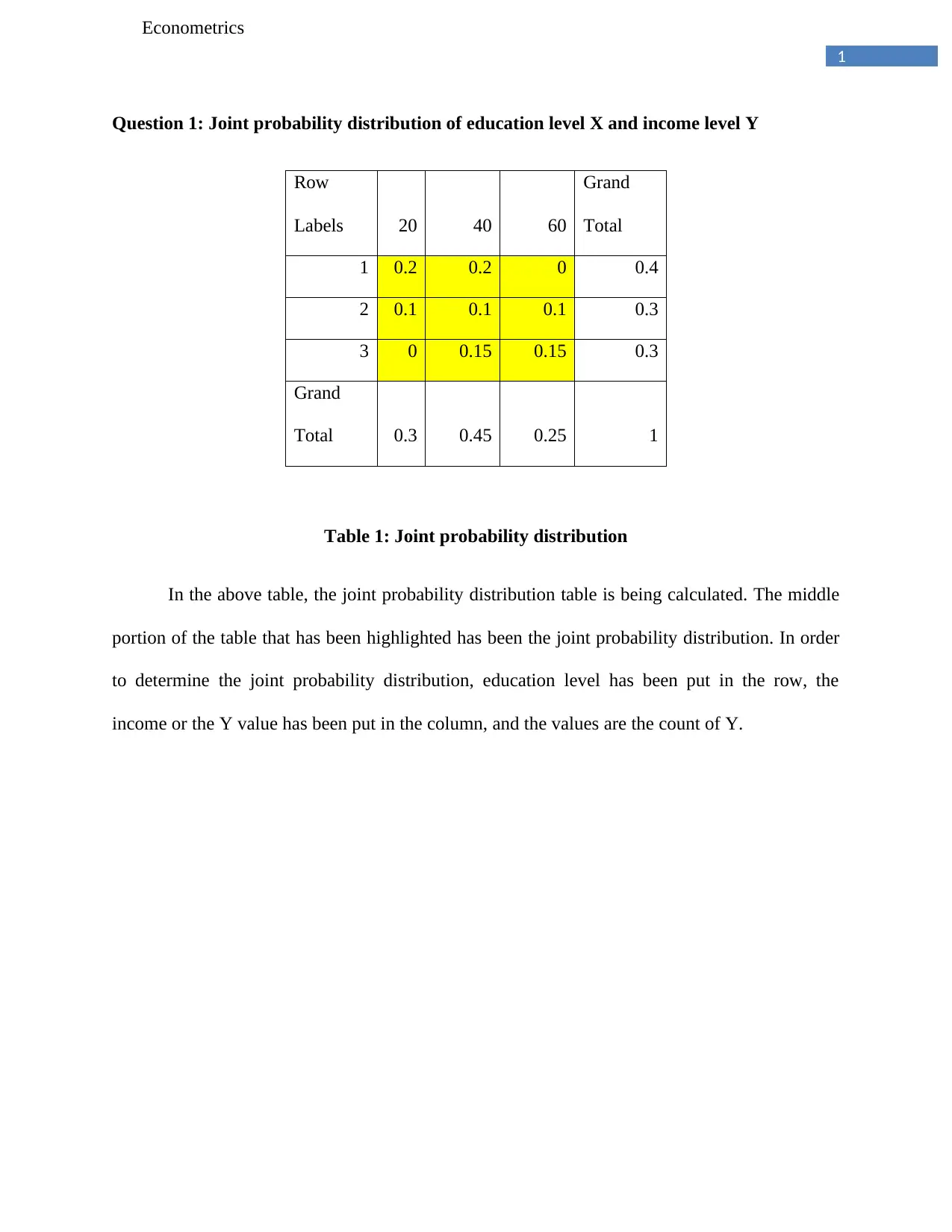
Question 1: Joint probability distribution of education level X and income level Y
Row
Labels 20 40 60
Grand
Total
1 0.2 0.2 0 0.4
2 0.1 0.1 0.1 0.3
3 0 0.15 0.15 0.3
Grand
Total 0.3 0.45 0.25 1
Table 1: Joint probability distribution
In the above table, the joint probability distribution table is being calculated. The middle
portion of the table that has been highlighted has been the joint probability distribution. In order
to determine the joint probability distribution, education level has been put in the row, the
income or the Y value has been put in the column, and the values are the count of Y.

2
Econometrics
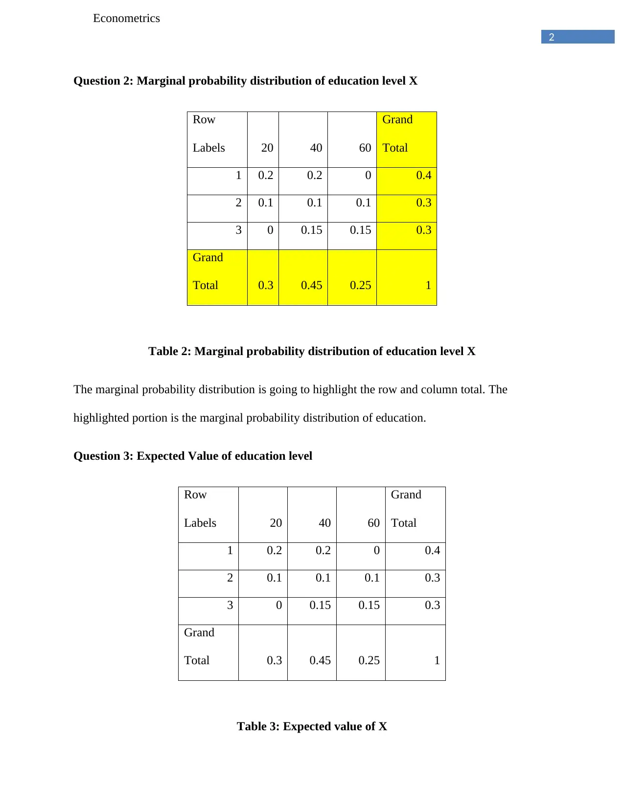
Question 2: Marginal probability distribution of education level X
Row
Labels 20 40 60
Grand
Total
1 0.2 0.2 0 0.4
2 0.1 0.1 0.1 0.3
3 0 0.15 0.15 0.3
Grand
Total 0.3 0.45 0.25 1
Table 2: Marginal probability distribution of education level X
The marginal probability distribution is going to highlight the row and column total. The
highlighted portion is the marginal probability distribution of education.
Question 3: Expected Value of education level
Row
Labels 20 40 60
Grand
Total
1 0.2 0.2 0 0.4
2 0.1 0.1 0.1 0.3
3 0 0.15 0.15 0.3
Grand
Total 0.3 0.45 0.25 1
Table 3: Expected value of X

3
Econometrics
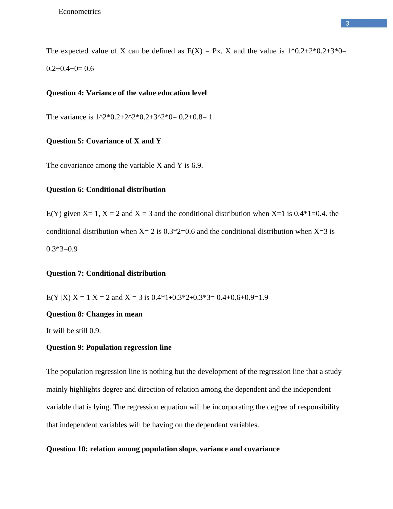
The expected value of X can be defined as E(X) = Px. X and the value is 1*0.2+2*0.2+3*0=
0.2+0.4+0= 0.6
Question 4: Variance of the value education level
The variance is 1^2*0.2+2^2*0.2+3^2*0= 0.2+0.8= 1
Question 5: Covariance of X and Y
The covariance among the variable X and Y is 6.9.
Question 6: Conditional distribution
E(Y) given X= 1, X = 2 and X = 3 and the conditional distribution when X=1 is 0.4*1=0.4. the
conditional distribution when X= 2 is 0.3*2=0.6 and the conditional distribution when X=3 is
0.3*3=0.9
Question 7: Conditional distribution
E(Y |X) X = 1 X = 2 and X = 3 is 0.4*1+0.3*2+0.3*3= 0.4+0.6+0.9=1.9
Question 8: Changes in mean
It will be still 0.9.
Question 9: Population regression line
The population regression line is nothing but the development of the regression line that a study
mainly highlights degree and direction of relation among the dependent and the independent
variable that is lying. The regression equation will be incorporating the degree of responsibility
that independent variables will be having on the dependent variables.
Question 10: relation among population slope, variance and covariance

4
Econometrics
Population slope is highlighting the fact that the tangent of the slope intercepts that will
definitely allow the curve to identify the direction of the regression. The population slope β will
determine the development of the prediction and that will definitely increase the prediction
regarding the development of the future trends and the estimated OLS regression that will allow
the prediction of the model in an effective and innovative manner. The variance will be looking
for the mean and they will be allowing the model to increase the improvement in the allocation
of the data. The covariance will be looking for the correlation and the inter dependence among
the dependent and independent variable and the model will be able to predict the goodness of fit
of the model.
Question 11: Dependent or independent of the variables
Both the variables X that is denoting the level of education and the variable Y is denoting the
level of the income. Both of these two variables are dependent to each other in the sense that
level of the education level will determine the income that the employees will be earning. The
two variables are having high chance of getting highly significant correlation variable.
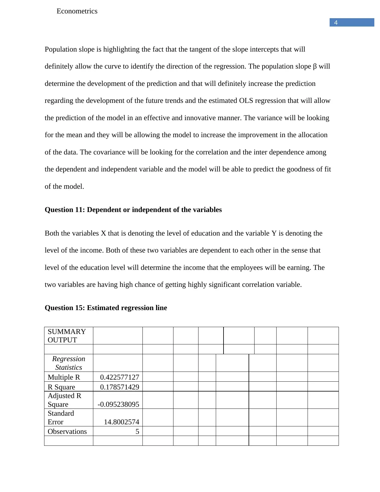
Question 15: Estimated regression line
SUMMARY
OUTPUT
Regression
Statistics
Multiple R 0.422577127
R Square 0.178571429
Adjusted R
Square -0.095238095
Standard
Error 14.8002574
Observations 5

5
Econometrics
ANOVA
df SS MS F
Signific
ance F
Regression 1
142.85
71429
142.8
5714
29
0.6
52
17
39
0.47843
02
Residual 3
657.14
28571
219.0
4761
9
Total 4 800
Coefficients
Standar
d Error t Stat
P-
val
ue
Lower
95%
Upper
95%
Lower
99.0%
Upper
99.0%
Intercept 24.28571429
20.553
56367
1.181
5816
8
0.3
22
50
52
-
41.1249
89.696
327
-
95.7657
9
144.337
2157
Xi 7.142857143
8.8448
45534
0.807
5728
53
0.4
78
43
02
-
21.0053
9
35.291
103
-
44.5190
8
58.8047
9776
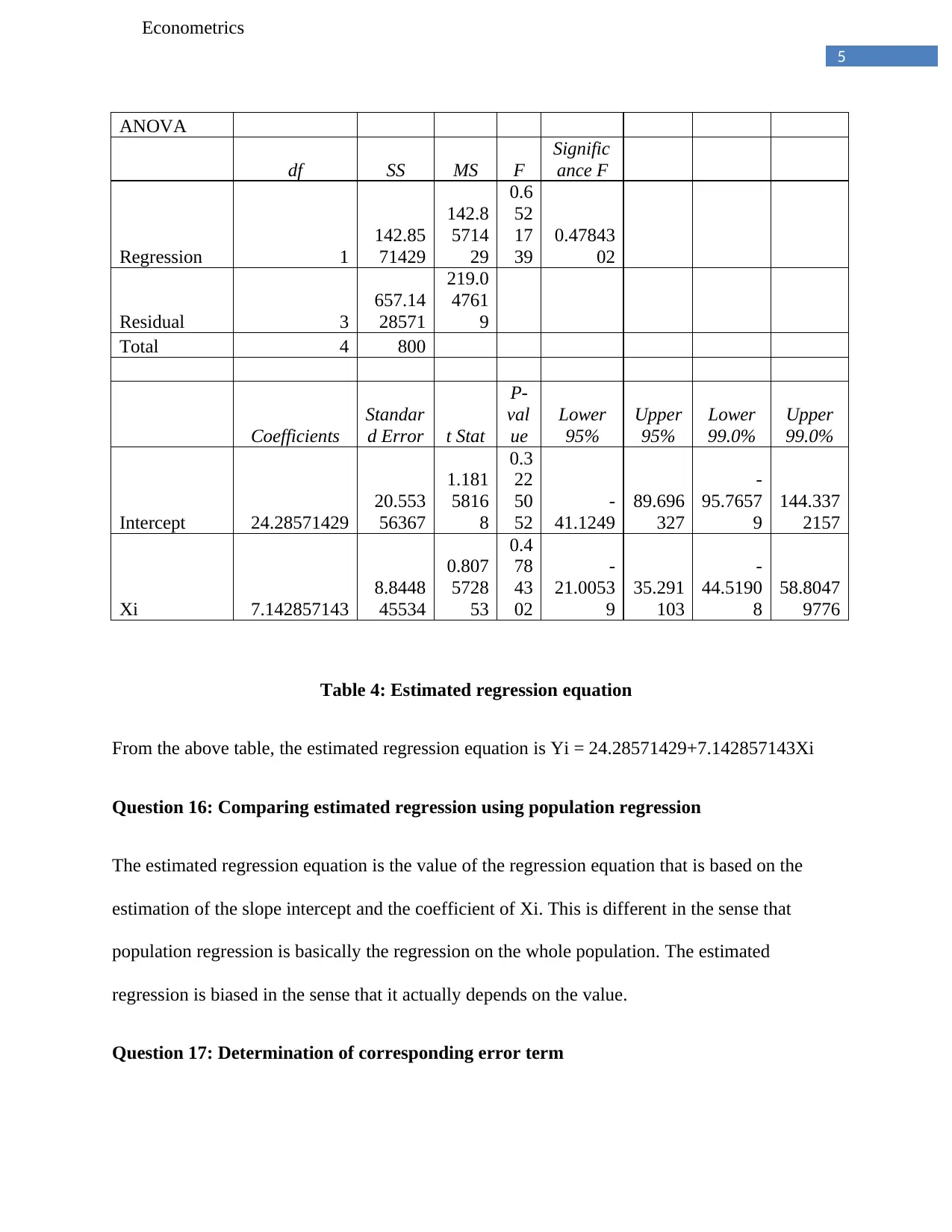
Table 4: Estimated regression equation
From the above table, the estimated regression equation is Yi = 24.28571429+7.142857143Xi
Question 16: Comparing estimated regression using population regression
The estimated regression equation is the value of the regression equation that is based on the
estimation of the slope intercept and the coefficient of Xi. This is different in the sense that
population regression is basically the regression on the whole population. The estimated
regression is biased in the sense that it actually depends on the value.
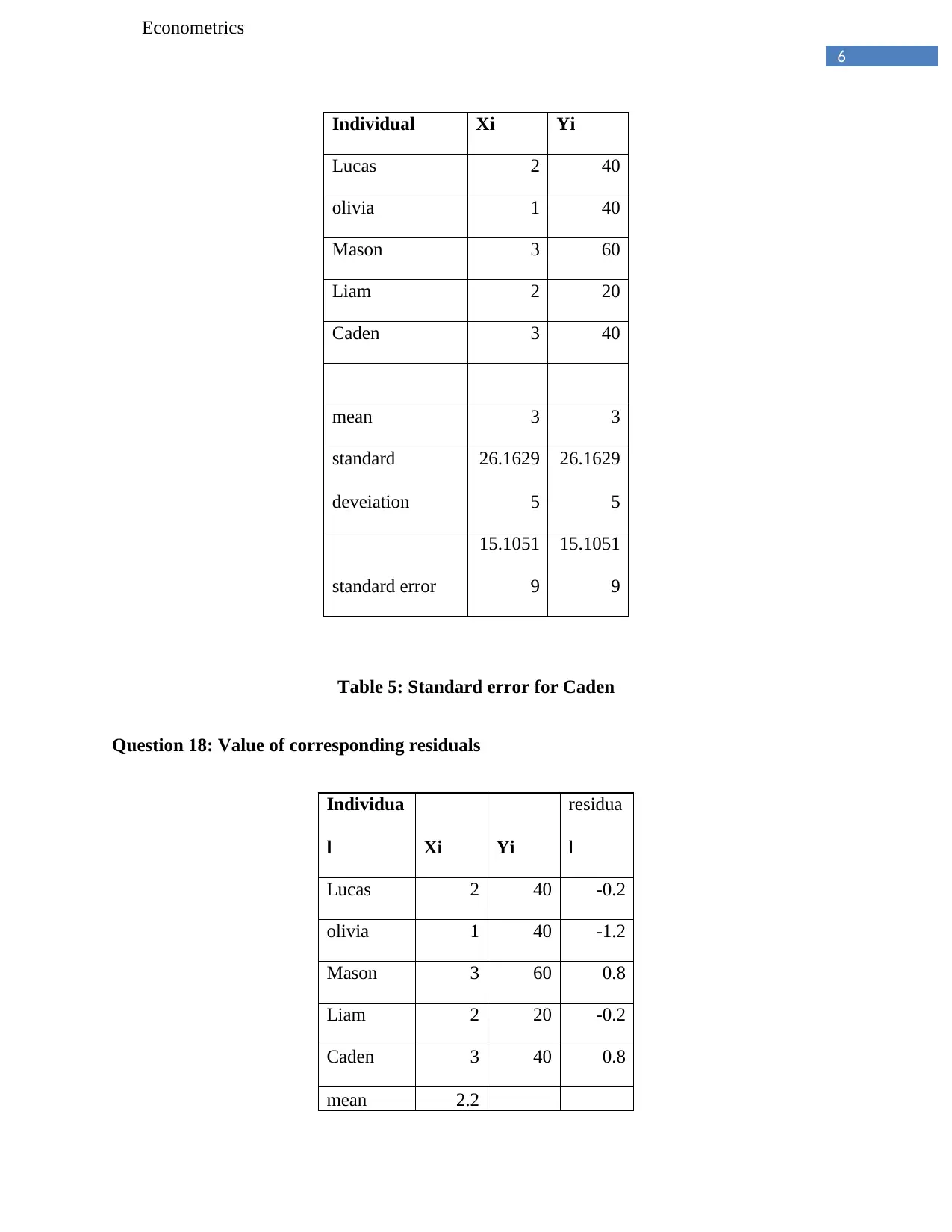
Question 17: Determination of corresponding error term

6
Econometrics
Individual Xi Yi
Lucas 2 40
olivia 1 40
Mason 3 60
Liam 2 20
Caden 3 40
mean 3 3
standard
deveiation
26.1629
5
26.1629
5
standard error
15.1051
9
15.1051
9
Table 5: Standard error for Caden
Question 18: Value of corresponding residuals
Individua
l Xi Yi
residua
l
Lucas 2 40 -0.2
olivia 1 40 -1.2
Mason 3 60 0.8
Liam 2 20 -0.2
Caden 3 40 0.8
mean 2.2

7
Econometrics

8
Econometrics
Bibliography
Bell, A. and Jones, K., 2015. Explaining fixed effects: Random effects modeling of time-series
cross-sectional and panel data. Political Science Research and Methods, 3(1), pp.133-153.
Bun, M.J. and Sarafidis, V., 2015. Dynamic panel data models. The oxford handbook of panel
data, pp.76-110.
Frühwirth-Schnatter, S., 2018. Bayesian Econometrics in the Big Data Era.
Lopez, L. and Weber, S., 2018. Testing for Granger causality in panel data. The Stata
Journal, 17(4), pp.972-984.
Stock, J.H. and Watson, M.W., 2015. Introduction to econometrics.