Statistical Data Collection and Interpretation for Energy Use in Australia
VerifiedAdded on 2023/06/14
|20
|3838
|388
AI Summary
This research study analyses the energy consumption data for different sectors in Australia using statistical data analysis. It aims to find out significant differences in energy use for different sectors, trends in energy use, and relationships between energy uses for different sectors. The study includes descriptive statistics, graphical analysis, correlation and regression analysis, independent samples t-tests, and one way ANOVA.
Contribute Materials
Your contribution can guide someone’s learning journey. Share your
documents today.
Statistical Data Collection and Interpretation
Assessment Item 3
Assessment Item 3
Secure Best Marks with AI Grader
Need help grading? Try our AI Grader for instant feedback on your assignments.
Table of Contents
Abstract................................................................................................................................3
Introduction..........................................................................................................................3
Research Questions..............................................................................................................4
Data Collection.....................................................................................................................5
Descriptive Statistics............................................................................................................4
Graphical Analysis...............................................................................................................5
Correlation and Regression Analysis...................................................................................3
Independent Samples t-tests.................................................................................................3
One way ANOVA................................................................................................................4
Results and Discussions.......................................................................................................4
Conclusions..........................................................................................................................5
References............................................................................................................................5
2 | P a g e
Assessment Item 3
Statistical Data Collection and Interpretation
Abstract
It is observed that average energy use for different sectors in Australia is not same. It is observed
that manufacturing sector needs most of the energy. Most significant sectors for energy uses are
given as manufacturing, electricity generation, transport, and residential. It is observed that the
energy use for the country is continuous increasing from the last 42 years. It is observed that
there is perfect linear relationship exists between the dependent variable and independent
variable for this regression model. There is sufficient evidence to conclude that there is a
statistically significant linear relationship exists between the dependent variable and independent
variables. There is insufficient evidence to conclude that there is a statistically significant
difference in the average energy use for the two sectors manufacturing and transport. There is
sufficient evidence to conclude that there is a significant difference in the average energy uses
for three sectors such as manufacturing, transport, and electricity generation.
Introduction
Statistical data analysis plays an important role in analysing different facts regarding the
business, industry, management, and many more sectors. Statistical analysis for any type of data
is the key for making effective decisions (Hogg, 2004). It helps in making effective decisions
and management according to analysis. Statistical data analysis helps in understand the actual
facts and it improves the creativity of managers (Degroot, 2002). For this research study, we
have to use statistical data analysis for the analysis of energy consumption data for the different
sectors in the Australia. By using this statistical data analysis we have to find out whether there
are any significant differences in the use of energy for the different sectors. Also, we want to
check the different trends in the energy uses in accordance with time factors. We will compare
different sectors for their energy uses and also we will study it for the entire use of energy for the
country. Let us see this research study in detail.
Research Questions
For this statistical data collection and analysis, the research questions are summarised as below:
1. Is there any significant differences observed between the different sectors for energy uses
in Australia?
2. What is the trend of energy uses in Australia for different sectors?
3. Is there any significant relationship exists between the energy uses for the different
sectors?
3 | P a g e
4. Is there a sufficient evidence to conclude that there is a statistically significant linear
relationship exists between the dependent variable and independent variables?
5. Is there a sufficient evidence to conclude that there is a statistically significant difference
in the average energy use for the two sectors manufacturing and transport?
6. Is there a sufficient evidence to conclude that there is a significant difference in the
average energy uses for three sectors such as manufacturing, transport, and electricity
generation?
Data Collection
For the study of above research questions, it is required to collect the data for the study variables.
For this research study, a data is collected from the government website (www.industry.gov.au)
of Department of Industry, Innovation and Science, Australia Government. A data is collected
for the 42 years for the energy uses for different sectors in the Australia. A proper method of the
data collection should use for getting unbiased results (Dobson, 2001). Instrumental errors
should be minimized and other chance causes should be at minimum level during the conduction
of research study (Casella, 2002). Using a data from secondary sources, proper care should be
taken while sampling with data (Hastle, 2001). A data link for more detail is provided in the
reference section. Data is given for the energy uses for different sectors such as agriculture,
mining, manufacturing, electricity generation, construction, transport, commercial, residential,
other sectors, etc. A screenshot of partial data is provided in the appendix section for more detail.
Descriptive Statistics
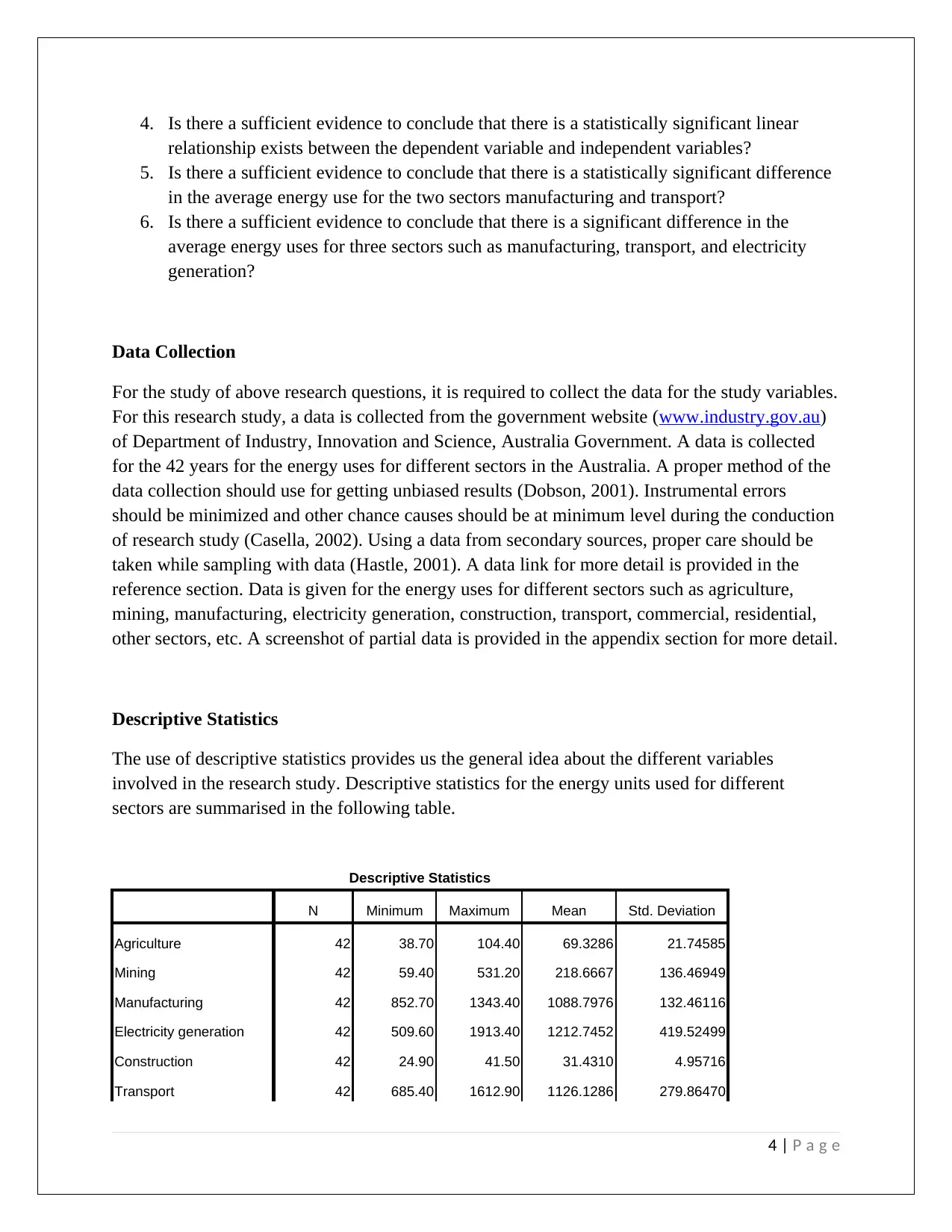
The use of descriptive statistics provides us the general idea about the different variables
involved in the research study. Descriptive statistics for the energy units used for different
sectors are summarised in the following table.
Descriptive Statistics
N Minimum Maximum Mean Std. Deviation
Agriculture 42 38.70 104.40 69.3286 21.74585
Mining 42 59.40 531.20 218.6667 136.46949
Manufacturing 42 852.70 1343.40 1088.7976 132.46116
Electricity generation 42 509.60 1913.40 1212.7452 419.52499
Construction 42 24.90 41.50 31.4310 4.95716
Transport 42 685.40 1612.90 1126.1286 279.86470
4 | P a g e
relationship exists between the dependent variable and independent variables?
5. Is there a sufficient evidence to conclude that there is a statistically significant difference
in the average energy use for the two sectors manufacturing and transport?
6. Is there a sufficient evidence to conclude that there is a significant difference in the
average energy uses for three sectors such as manufacturing, transport, and electricity
generation?
Data Collection
For the study of above research questions, it is required to collect the data for the study variables.
For this research study, a data is collected from the government website (www.industry.gov.au)
of Department of Industry, Innovation and Science, Australia Government. A data is collected
for the 42 years for the energy uses for different sectors in the Australia. A proper method of the
data collection should use for getting unbiased results (Dobson, 2001). Instrumental errors
should be minimized and other chance causes should be at minimum level during the conduction
of research study (Casella, 2002). Using a data from secondary sources, proper care should be
taken while sampling with data (Hastle, 2001). A data link for more detail is provided in the
reference section. Data is given for the energy uses for different sectors such as agriculture,
mining, manufacturing, electricity generation, construction, transport, commercial, residential,
other sectors, etc. A screenshot of partial data is provided in the appendix section for more detail.
Descriptive Statistics
The use of descriptive statistics provides us the general idea about the different variables
involved in the research study. Descriptive statistics for the energy units used for different
sectors are summarised in the following table.
Descriptive Statistics
N Minimum Maximum Mean Std. Deviation
Agriculture 42 38.70 104.40 69.3286 21.74585
Mining 42 59.40 531.20 218.6667 136.46949
Manufacturing 42 852.70 1343.40 1088.7976 132.46116
Electricity generation 42 509.60 1913.40 1212.7452 419.52499
Construction 42 24.90 41.50 31.4310 4.95716
Transport 42 685.40 1612.90 1126.1286 279.86470
4 | P a g e
Secure Best Marks with AI Grader
Need help grading? Try our AI Grader for instant feedback on your assignments.
Commercial 42 84.50 336.20 190.3690 80.21346
Residential 42 231.30 456.00 350.4024 72.62252
Other 42 48.20 102.00 70.8500 11.54149
Total 42 2615.20 5953.80 4358.7190 1119.80978
Valid N (listwise) 42
From above table, it is observed that average energy use for agriculture sector for Australia is
given as 69.33 energy units with the standard deviation of 21.75 energy units. It is seen that
average total energy use for Australia is given as 4358.71 energy units with the standard
deviation of 1119.81 energy units. From the given table, it is observed that manufacturing sector
needs most of the energy. Most significant sectors for energy uses are given as manufacturing,
electricity generation, transport, and residential.
Graphical Analysis
Graphical analysis of the data provides an easy idea for comparisons and understanding of the
concepts (Evans, 2004). Now, we have to see some graphical analysis for the given information
regarding the energy uses in Australia.
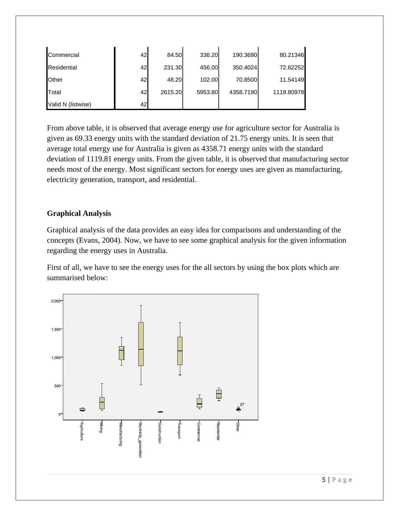
First of all, we have to see the energy uses for the all sectors by using the box plots which are
summarised below:
5 | P a g e
Residential 42 231.30 456.00 350.4024 72.62252
Other 42 48.20 102.00 70.8500 11.54149
Total 42 2615.20 5953.80 4358.7190 1119.80978
Valid N (listwise) 42
From above table, it is observed that average energy use for agriculture sector for Australia is
given as 69.33 energy units with the standard deviation of 21.75 energy units. It is seen that
average total energy use for Australia is given as 4358.71 energy units with the standard
deviation of 1119.81 energy units. From the given table, it is observed that manufacturing sector
needs most of the energy. Most significant sectors for energy uses are given as manufacturing,
electricity generation, transport, and residential.
Graphical Analysis
Graphical analysis of the data provides an easy idea for comparisons and understanding of the
concepts (Evans, 2004). Now, we have to see some graphical analysis for the given information
regarding the energy uses in Australia.
First of all, we have to see the energy uses for the all sectors by using the box plots which are
summarised below:
5 | P a g e
From the given box plots, it is observed that the energy use for the sectors manufacturing,
electricity generation, and transport is high as compare to other sectors, agriculture and
construction uses less energy.
Now, we have to see some time series analysis for the energy uses for different sectors for the
last 40 years.
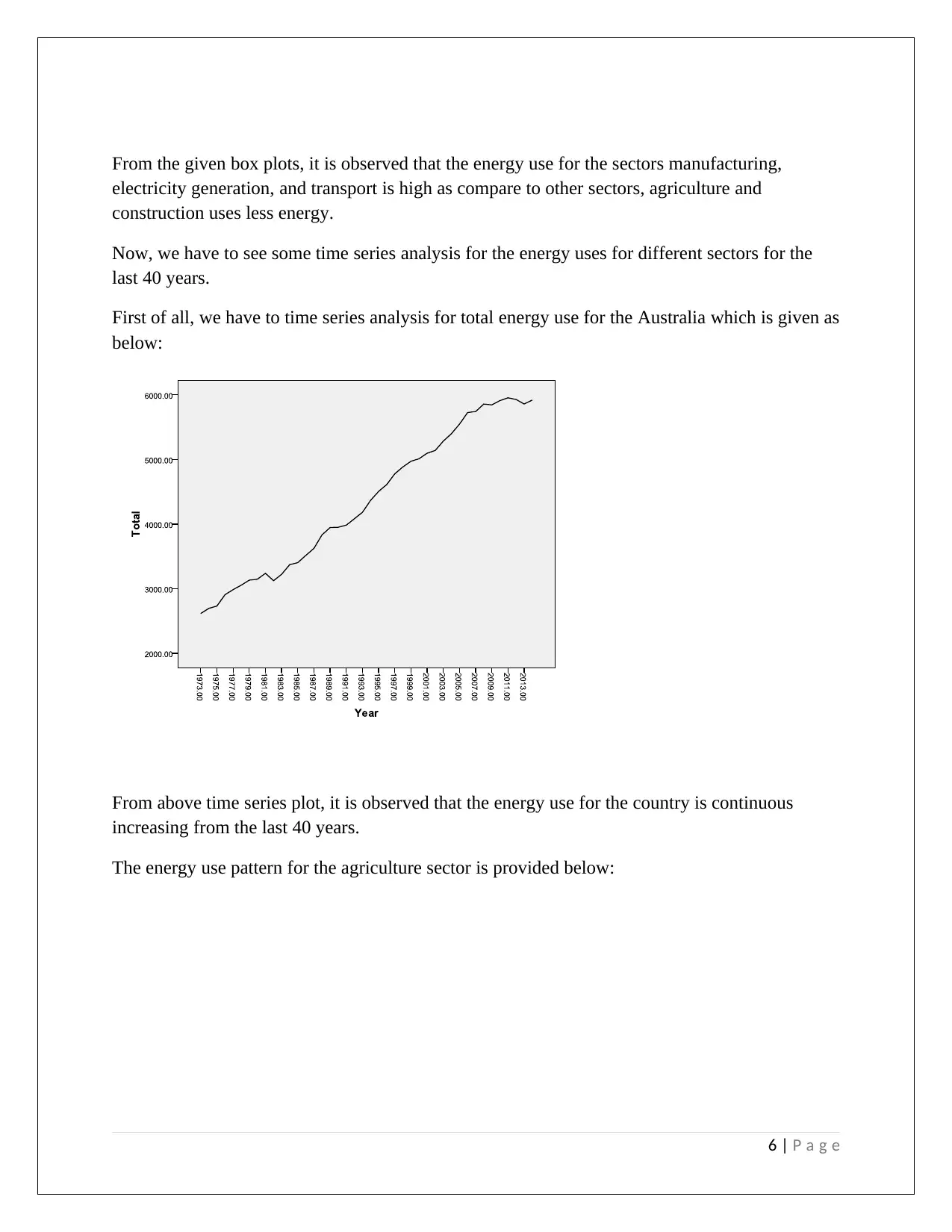
First of all, we have to time series analysis for total energy use for the Australia which is given as
below:
From above time series plot, it is observed that the energy use for the country is continuous
increasing from the last 40 years.
The energy use pattern for the agriculture sector is provided below:
6 | P a g e
electricity generation, and transport is high as compare to other sectors, agriculture and
construction uses less energy.
Now, we have to see some time series analysis for the energy uses for different sectors for the
last 40 years.
First of all, we have to time series analysis for total energy use for the Australia which is given as
below:
From above time series plot, it is observed that the energy use for the country is continuous
increasing from the last 40 years.
The energy use pattern for the agriculture sector is provided below:
6 | P a g e
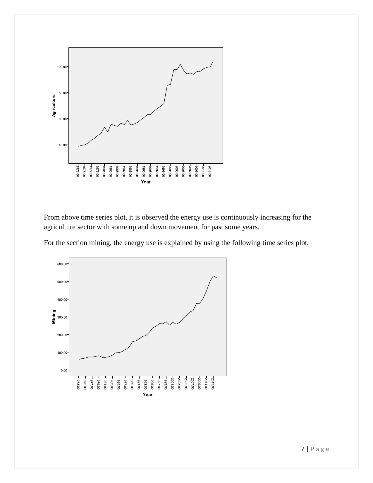
From above time series plot, it is observed the energy use is continuously increasing for the
agriculture sector with some up and down movement for past some years.
For the section mining, the energy use is explained by using the following time series plot.
7 | P a g e
agriculture sector with some up and down movement for past some years.
For the section mining, the energy use is explained by using the following time series plot.
7 | P a g e
Paraphrase This Document
Need a fresh take? Get an instant paraphrase of this document with our AI Paraphraser
From above given time series plot, it is observed that the energy use for the mining sector is
continuously increasing.
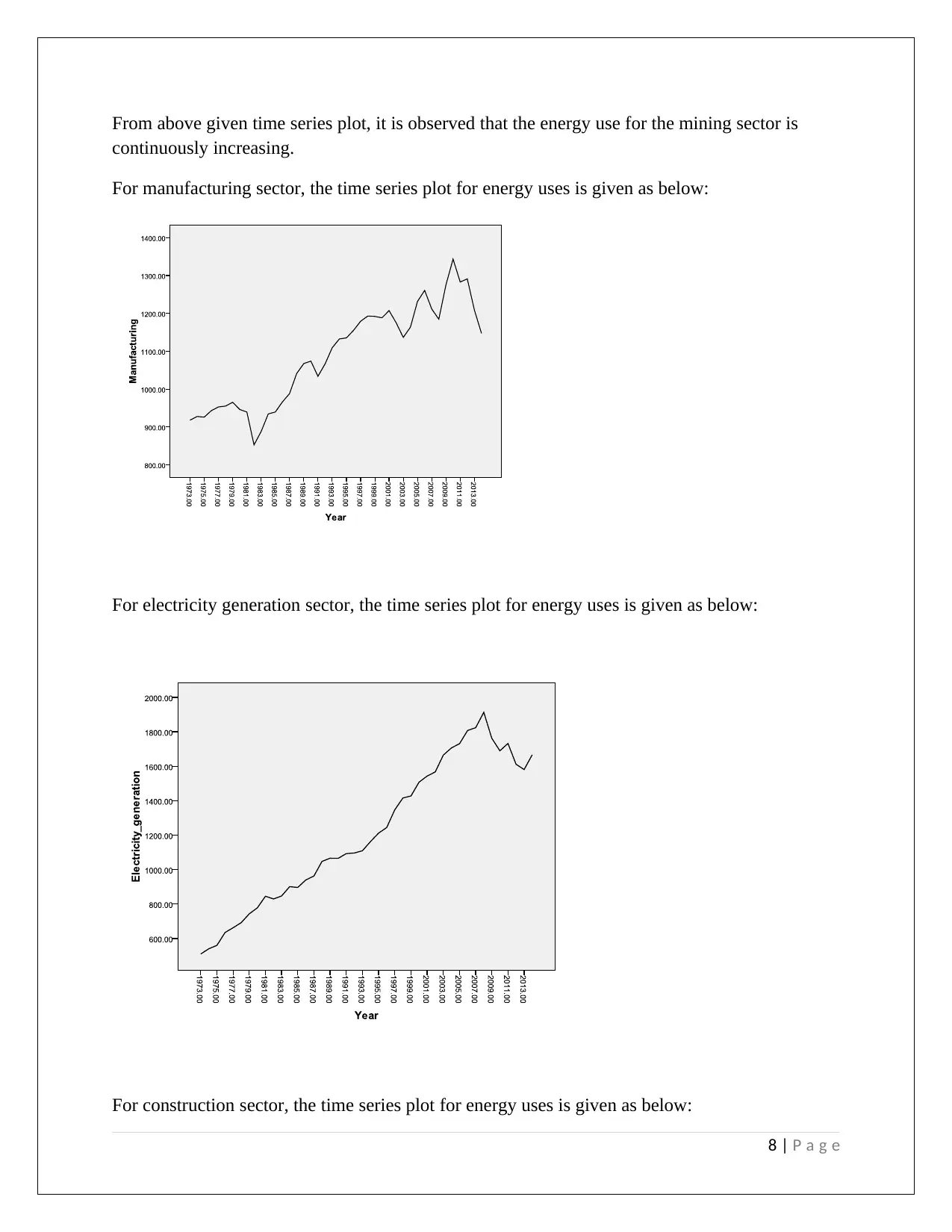
For manufacturing sector, the time series plot for energy uses is given as below:
For electricity generation sector, the time series plot for energy uses is given as below:
For construction sector, the time series plot for energy uses is given as below:
8 | P a g e
continuously increasing.
For manufacturing sector, the time series plot for energy uses is given as below:
For electricity generation sector, the time series plot for energy uses is given as below:
For construction sector, the time series plot for energy uses is given as below:
8 | P a g e
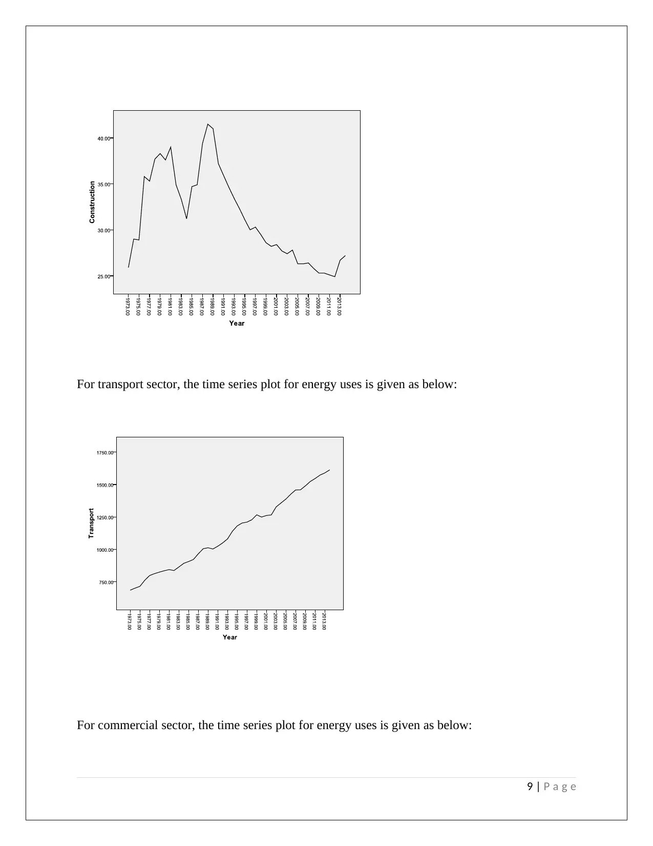
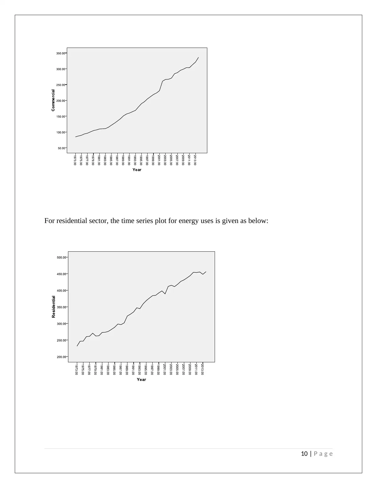
For transport sector, the time series plot for energy uses is given as below:
For commercial sector, the time series plot for energy uses is given as below:
9 | P a g e
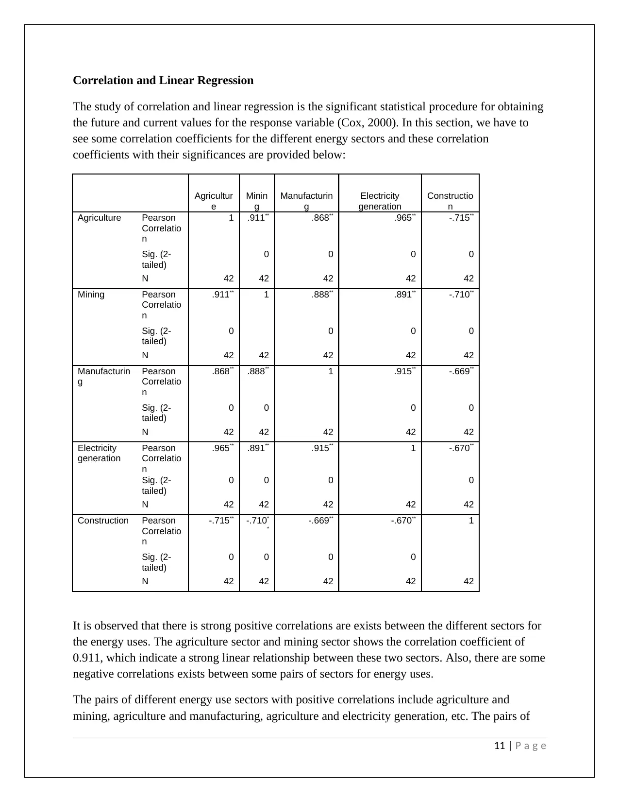
For commercial sector, the time series plot for energy uses is given as below:
9 | P a g e
For residential sector, the time series plot for energy uses is given as below:
10 | P a g e
10 | P a g e
Secure Best Marks with AI Grader
Need help grading? Try our AI Grader for instant feedback on your assignments.
Correlation and Linear Regression
The study of correlation and linear regression is the significant statistical procedure for obtaining
the future and current values for the response variable (Cox, 2000). In this section, we have to
see some correlation coefficients for the different energy sectors and these correlation
coefficients with their significances are provided below:
Agricultur
e
Minin
g
Manufacturin
g
Electricity
generation
Constructio
n
Agriculture Pearson
Correlatio
n
1 .911** .868** .965** -.715**
Sig. (2-
tailed)
0 0 0 0
N 42 42 42 42 42
Mining Pearson
Correlatio
n
.911** 1 .888** .891** -.710**
Sig. (2-
tailed)
0 0 0 0
N 42 42 42 42 42
Manufacturin
g
Pearson
Correlatio
n
.868** .888** 1 .915** -.669**
Sig. (2-
tailed)
0 0 0 0
N 42 42 42 42 42
Electricity
generation
Pearson
Correlatio
n
.965** .891** .915** 1 -.670**
Sig. (2-
tailed)
0 0 0 0
N 42 42 42 42 42
Construction Pearson
Correlatio
n
-.715** -.710*
*
-.669** -.670** 1
Sig. (2-
tailed)
0 0 0 0
N 42 42 42 42 42
It is observed that there is strong positive correlations are exists between the different sectors for
the energy uses. The agriculture sector and mining sector shows the correlation coefficient of
0.911, which indicate a strong linear relationship between these two sectors. Also, there are some
negative correlations exists between some pairs of sectors for energy uses.
The pairs of different energy use sectors with positive correlations include agriculture and
mining, agriculture and manufacturing, agriculture and electricity generation, etc. The pairs of
11 | P a g e
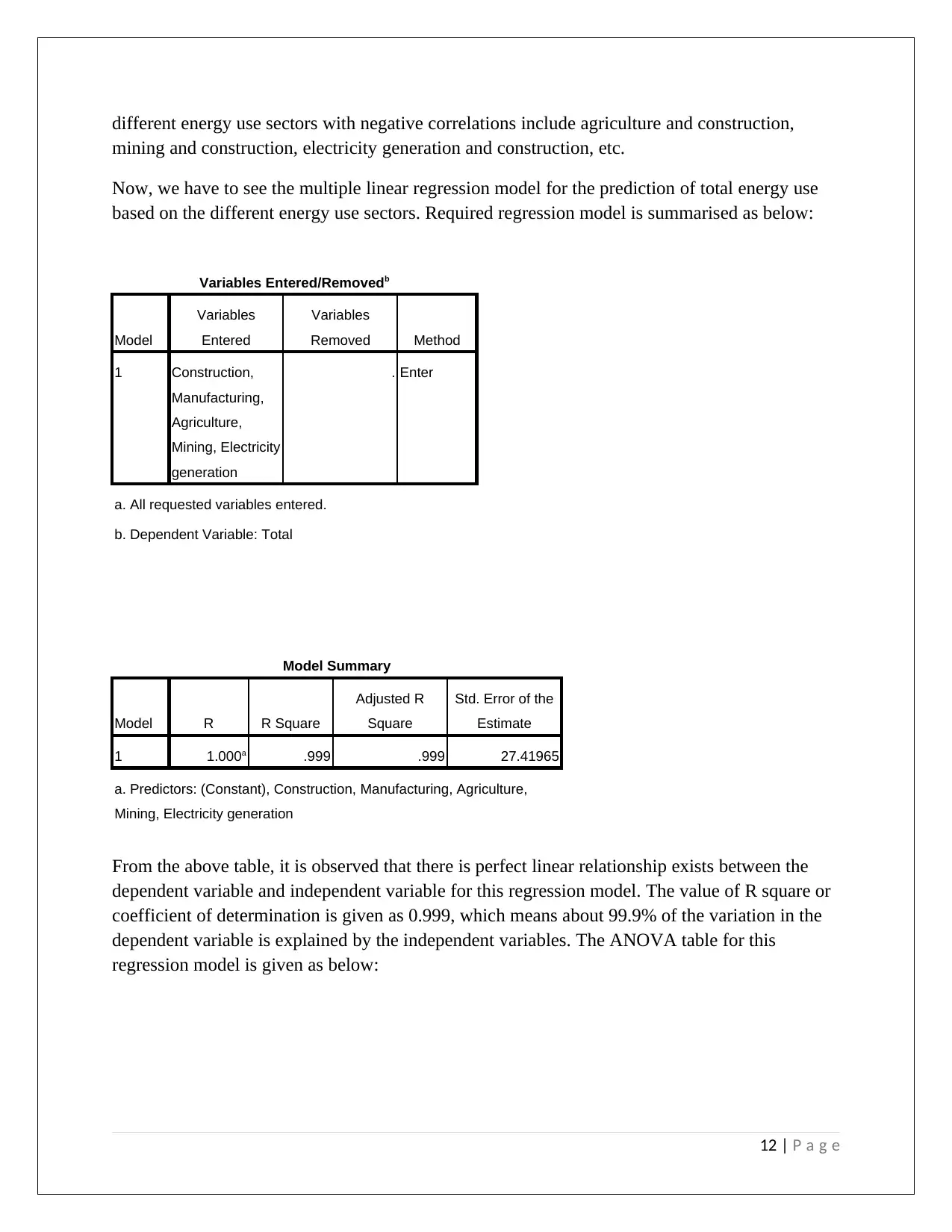
different energy use sectors with negative correlations include agriculture and construction,
mining and construction, electricity generation and construction, etc.
Now, we have to see the multiple linear regression model for the prediction of total energy use
based on the different energy use sectors. Required regression model is summarised as below:
Variables Entered/Removedb
Model
Variables
Entered
Variables
Removed Method
1 Construction,
Manufacturing,
Agriculture,
Mining, Electricity
generation
. Enter
a. All requested variables entered.
b. Dependent Variable: Total
Model Summary
Model R R Square
Adjusted R
Square
Std. Error of the
Estimate
1 1.000a .999 .999 27.41965
a. Predictors: (Constant), Construction, Manufacturing, Agriculture,
Mining, Electricity generation
From the above table, it is observed that there is perfect linear relationship exists between the
dependent variable and independent variable for this regression model. The value of R square or
coefficient of determination is given as 0.999, which means about 99.9% of the variation in the
dependent variable is explained by the independent variables. The ANOVA table for this
regression model is given as below:
12 | P a g e
ANOVAb
Model Sum of Squares df Mean Square F Sig.
1 Regression 5.139E7 5 1.028E7 13669.409 .000a
Residual 27066.148 36 751.837
Total 5.141E7 41
a. Predictors: (Constant), Construction, Manufacturing, Agriculture, Mining, Electricity generation
b. Dependent Variable: Total
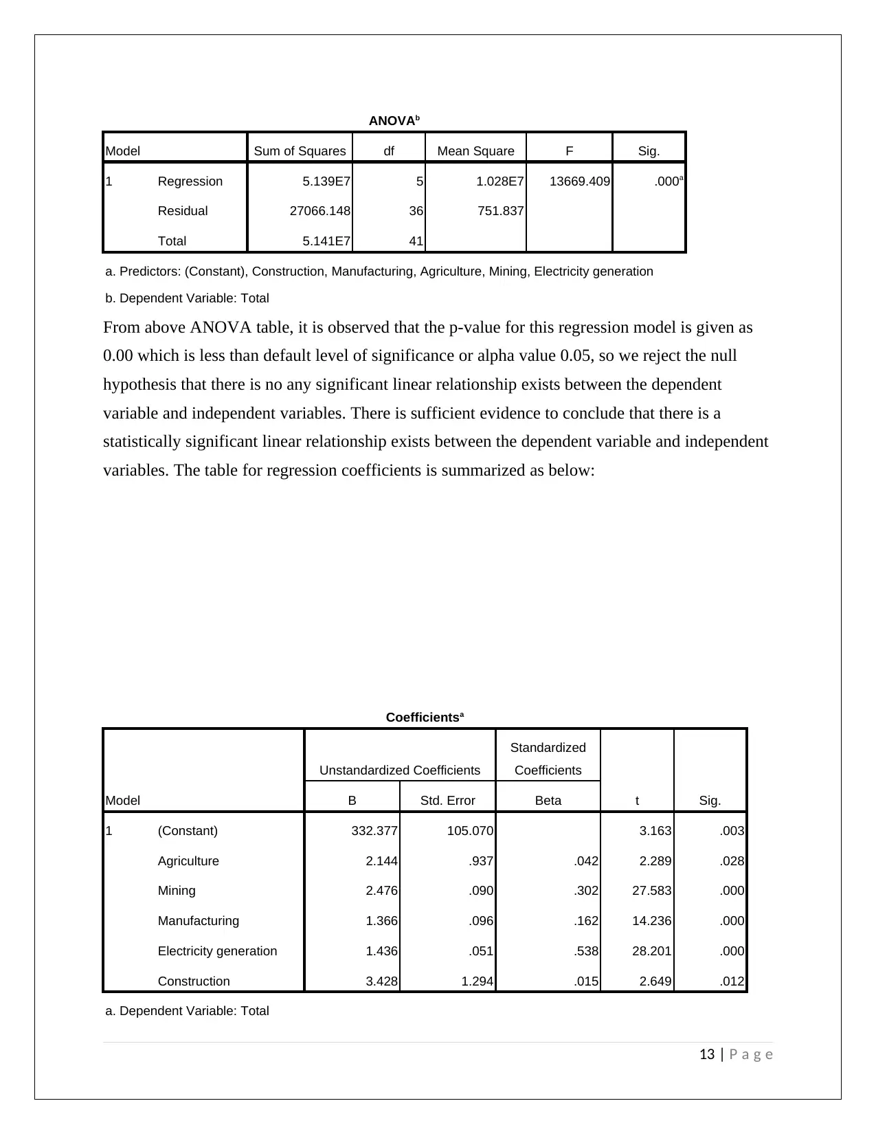
From above ANOVA table, it is observed that the p-value for this regression model is given as
0.00 which is less than default level of significance or alpha value 0.05, so we reject the null
hypothesis that there is no any significant linear relationship exists between the dependent
variable and independent variables. There is sufficient evidence to conclude that there is a
statistically significant linear relationship exists between the dependent variable and independent
variables. The table for regression coefficients is summarized as below:
Coefficientsa
Model
Unstandardized Coefficients
Standardized
Coefficients
t Sig.B Std. Error Beta
1 (Constant) 332.377 105.070 3.163 .003
Agriculture 2.144 .937 .042 2.289 .028
Mining 2.476 .090 .302 27.583 .000
Manufacturing 1.366 .096 .162 14.236 .000
Electricity generation 1.436 .051 .538 28.201 .000
Construction 3.428 1.294 .015 2.649 .012
a. Dependent Variable: Total
13 | P a g e
Model Sum of Squares df Mean Square F Sig.
1 Regression 5.139E7 5 1.028E7 13669.409 .000a
Residual 27066.148 36 751.837
Total 5.141E7 41
a. Predictors: (Constant), Construction, Manufacturing, Agriculture, Mining, Electricity generation
b. Dependent Variable: Total
From above ANOVA table, it is observed that the p-value for this regression model is given as
0.00 which is less than default level of significance or alpha value 0.05, so we reject the null
hypothesis that there is no any significant linear relationship exists between the dependent
variable and independent variables. There is sufficient evidence to conclude that there is a
statistically significant linear relationship exists between the dependent variable and independent
variables. The table for regression coefficients is summarized as below:
Coefficientsa
Model
Unstandardized Coefficients
Standardized
Coefficients
t Sig.B Std. Error Beta
1 (Constant) 332.377 105.070 3.163 .003
Agriculture 2.144 .937 .042 2.289 .028
Mining 2.476 .090 .302 27.583 .000
Manufacturing 1.366 .096 .162 14.236 .000
Electricity generation 1.436 .051 .538 28.201 .000
Construction 3.428 1.294 .015 2.649 .012
a. Dependent Variable: Total
13 | P a g e
Paraphrase This Document
Need a fresh take? Get an instant paraphrase of this document with our AI Paraphraser
Above regression coefficients are statistically significant as the corresponding p-values are less
than the level of significance or alpha value 0.05.
Independent Samples t-test
Testing hypothesis is the technique in inferential statistics which allow us for deciding whether
hypothesis would be rejected or not (Pearl, 2000). Statistical testing have a significant role in the
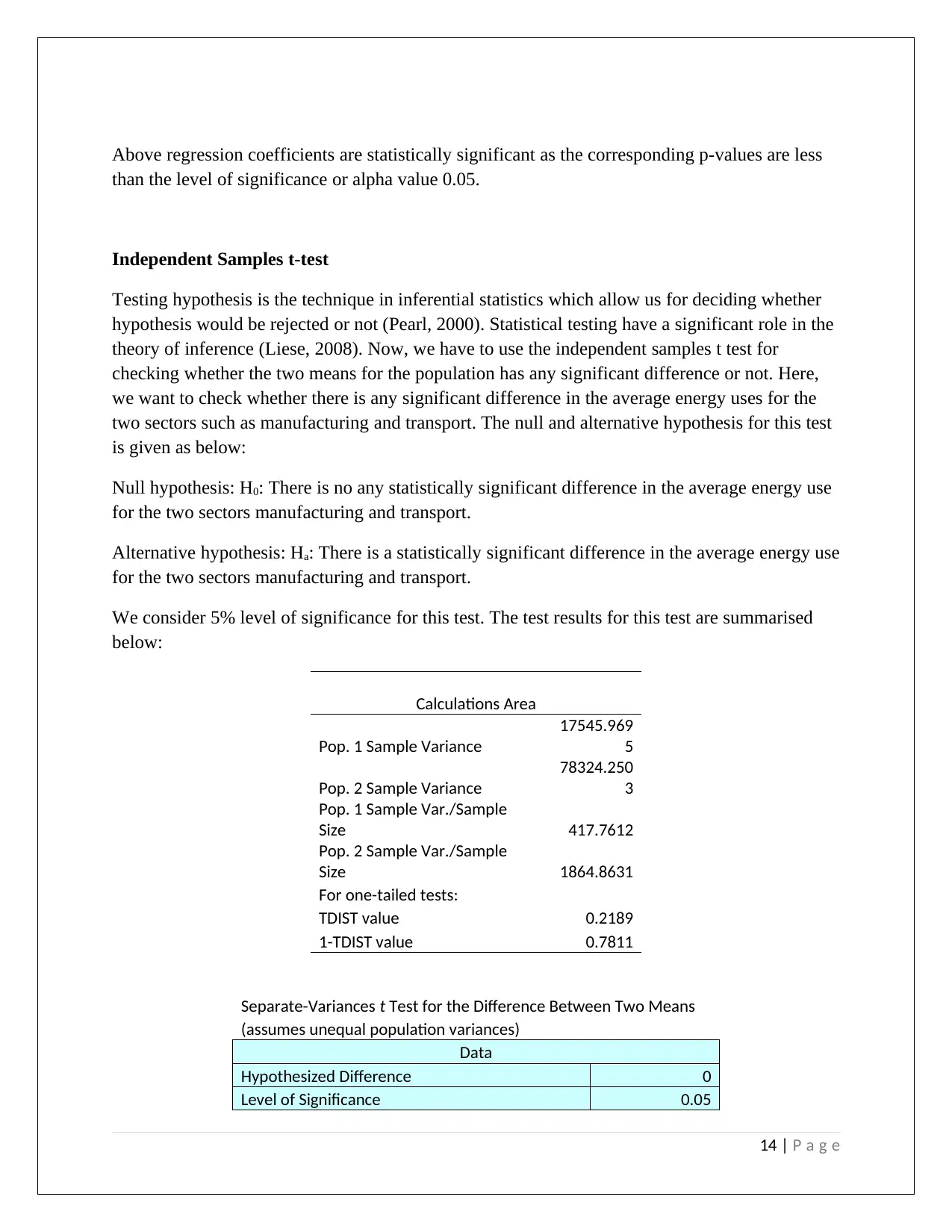
theory of inference (Liese, 2008). Now, we have to use the independent samples t test for
checking whether the two means for the population has any significant difference or not. Here,
we want to check whether there is any significant difference in the average energy uses for the
two sectors such as manufacturing and transport. The null and alternative hypothesis for this test
is given as below:
Null hypothesis: H0: There is no any statistically significant difference in the average energy use
for the two sectors manufacturing and transport.
Alternative hypothesis: Ha: There is a statistically significant difference in the average energy use
for the two sectors manufacturing and transport.
We consider 5% level of significance for this test. The test results for this test are summarised
below:
Calculations Area
Pop. 1 Sample Variance
17545.969
5
Pop. 2 Sample Variance
78324.250
3
Pop. 1 Sample Var./Sample
Size 417.7612
Pop. 2 Sample Var./Sample
Size 1864.8631
For one-tailed tests:
TDIST value 0.2189
1-TDIST value 0.7811
Separate-Variances t Test for the Difference Between Two Means
(assumes unequal population variances)
Data
Hypothesized Difference 0
Level of Significance 0.05
14 | P a g e
than the level of significance or alpha value 0.05.
Independent Samples t-test
Testing hypothesis is the technique in inferential statistics which allow us for deciding whether
hypothesis would be rejected or not (Pearl, 2000). Statistical testing have a significant role in the
theory of inference (Liese, 2008). Now, we have to use the independent samples t test for
checking whether the two means for the population has any significant difference or not. Here,
we want to check whether there is any significant difference in the average energy uses for the
two sectors such as manufacturing and transport. The null and alternative hypothesis for this test
is given as below:
Null hypothesis: H0: There is no any statistically significant difference in the average energy use
for the two sectors manufacturing and transport.
Alternative hypothesis: Ha: There is a statistically significant difference in the average energy use
for the two sectors manufacturing and transport.
We consider 5% level of significance for this test. The test results for this test are summarised
below:
Calculations Area
Pop. 1 Sample Variance
17545.969
5
Pop. 2 Sample Variance
78324.250
3
Pop. 1 Sample Var./Sample
Size 417.7612
Pop. 2 Sample Var./Sample
Size 1864.8631
For one-tailed tests:
TDIST value 0.2189
1-TDIST value 0.7811
Separate-Variances t Test for the Difference Between Two Means
(assumes unequal population variances)
Data
Hypothesized Difference 0
Level of Significance 0.05
14 | P a g e
Population 1 Sample
Sample Size 42
Sample Mean 1088.797619
Sample Standard Deviation 132.4612
Population 2 Sample
Sample Size 42
Sample Mean 1126.128571
Sample Standard Deviation 279.8647
Intermediate Calculations
Numerator of Degrees of Freedom 5210373.6950
Denominator of Degrees of Freedom 89078.9952
Total Degrees of Freedom 58.4916
Degrees of Freedom 58
Standard Error 47.7768
Difference in Sample Means -37.3310
Separate-Variance t Test Statistic -0.7814
Two-Tail Test
Lower Critical Value -2.0017
Upper Critical Value 2.0017
p-Value 0.4377
Do not reject the null hypothesis
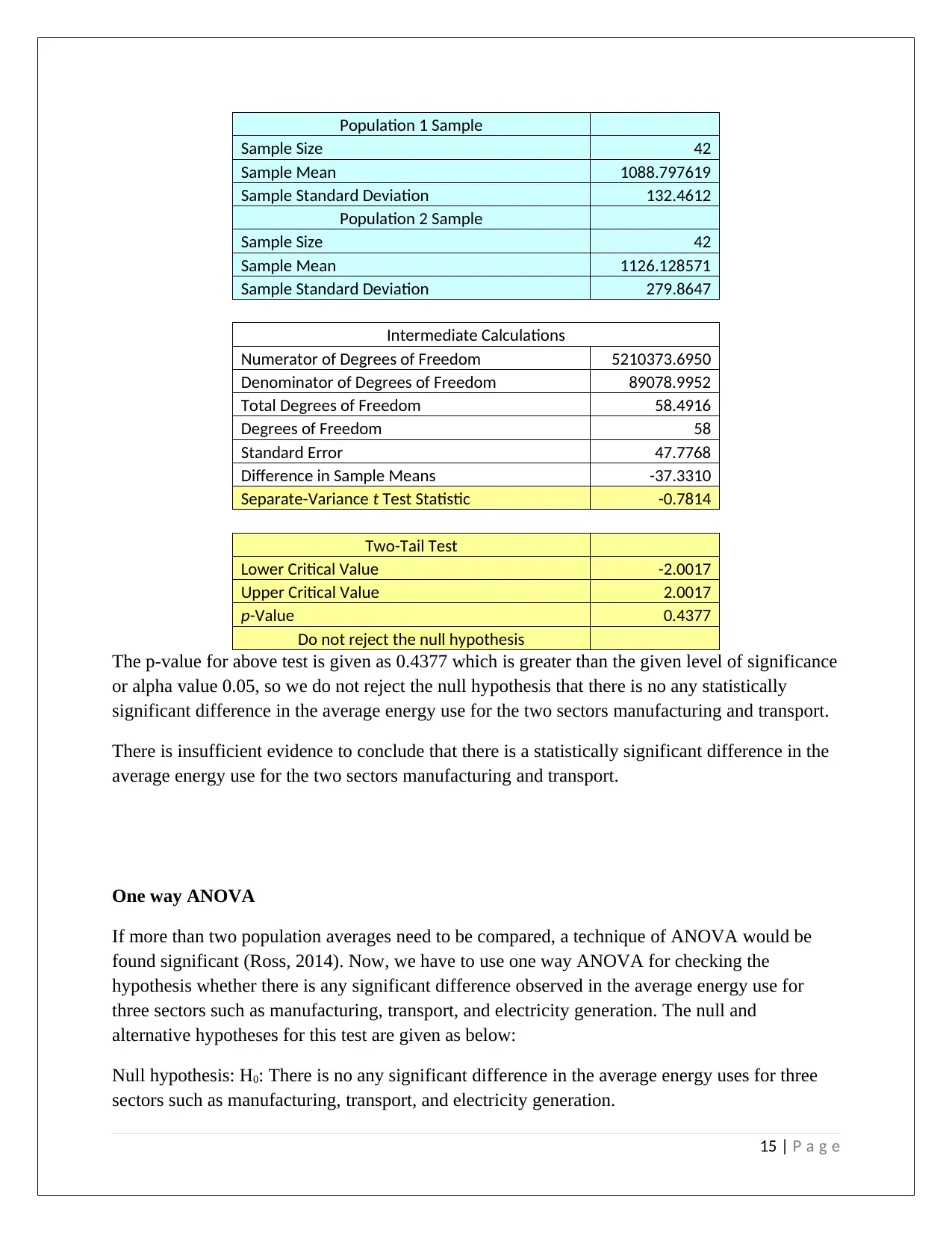
The p-value for above test is given as 0.4377 which is greater than the given level of significance
or alpha value 0.05, so we do not reject the null hypothesis that there is no any statistically
significant difference in the average energy use for the two sectors manufacturing and transport.
There is insufficient evidence to conclude that there is a statistically significant difference in the
average energy use for the two sectors manufacturing and transport.
One way ANOVA
If more than two population averages need to be compared, a technique of ANOVA would be
found significant (Ross, 2014). Now, we have to use one way ANOVA for checking the
hypothesis whether there is any significant difference observed in the average energy use for
three sectors such as manufacturing, transport, and electricity generation. The null and
alternative hypotheses for this test are given as below:
Null hypothesis: H0: There is no any significant difference in the average energy uses for three
sectors such as manufacturing, transport, and electricity generation.
15 | P a g e
Sample Size 42
Sample Mean 1088.797619
Sample Standard Deviation 132.4612
Population 2 Sample
Sample Size 42
Sample Mean 1126.128571
Sample Standard Deviation 279.8647
Intermediate Calculations
Numerator of Degrees of Freedom 5210373.6950
Denominator of Degrees of Freedom 89078.9952
Total Degrees of Freedom 58.4916
Degrees of Freedom 58
Standard Error 47.7768
Difference in Sample Means -37.3310
Separate-Variance t Test Statistic -0.7814
Two-Tail Test
Lower Critical Value -2.0017
Upper Critical Value 2.0017
p-Value 0.4377
Do not reject the null hypothesis
The p-value for above test is given as 0.4377 which is greater than the given level of significance
or alpha value 0.05, so we do not reject the null hypothesis that there is no any statistically
significant difference in the average energy use for the two sectors manufacturing and transport.
There is insufficient evidence to conclude that there is a statistically significant difference in the
average energy use for the two sectors manufacturing and transport.
One way ANOVA
If more than two population averages need to be compared, a technique of ANOVA would be
found significant (Ross, 2014). Now, we have to use one way ANOVA for checking the
hypothesis whether there is any significant difference observed in the average energy use for
three sectors such as manufacturing, transport, and electricity generation. The null and
alternative hypotheses for this test are given as below:
Null hypothesis: H0: There is no any significant difference in the average energy uses for three
sectors such as manufacturing, transport, and electricity generation.
15 | P a g e
Alternative hypothesis: Ha: There is a significant difference in the average energy uses for three
sectors such as manufacturing, transport, and electricity generation.
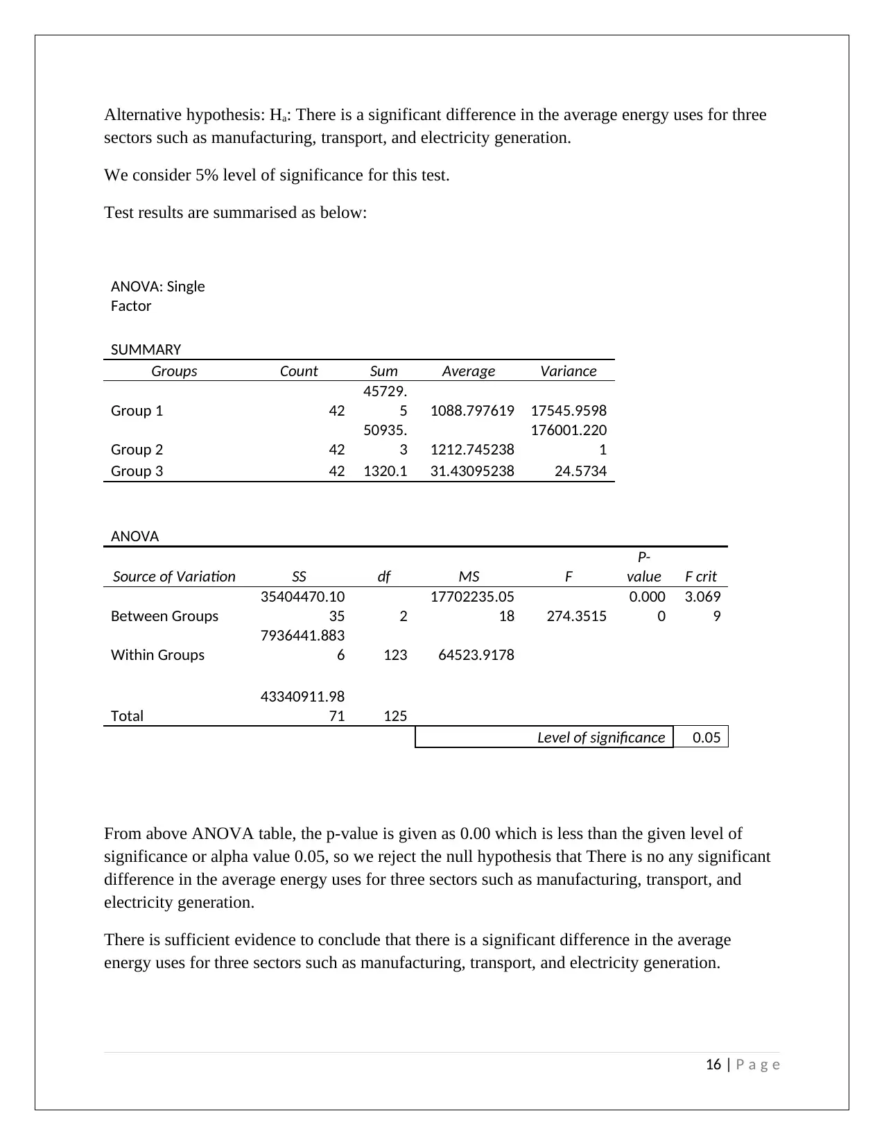
We consider 5% level of significance for this test.
Test results are summarised as below:
ANOVA: Single
Factor
SUMMARY
Groups Count Sum Average Variance
Group 1 42
45729.
5 1088.797619 17545.9598
Group 2 42
50935.
3 1212.745238
176001.220
1
Group 3 42 1320.1 31.43095238 24.5734
ANOVA
Source of Variation SS df MS F
P-
value F crit
Between Groups
35404470.10
35 2
17702235.05
18 274.3515
0.000
0
3.069
9
Within Groups
7936441.883
6 123 64523.9178
Total
43340911.98
71 125
Level of significance 0.05
From above ANOVA table, the p-value is given as 0.00 which is less than the given level of
significance or alpha value 0.05, so we reject the null hypothesis that There is no any significant
difference in the average energy uses for three sectors such as manufacturing, transport, and
electricity generation.
There is sufficient evidence to conclude that there is a significant difference in the average
energy uses for three sectors such as manufacturing, transport, and electricity generation.
16 | P a g e
sectors such as manufacturing, transport, and electricity generation.
We consider 5% level of significance for this test.
Test results are summarised as below:
ANOVA: Single
Factor
SUMMARY
Groups Count Sum Average Variance
Group 1 42
45729.
5 1088.797619 17545.9598
Group 2 42
50935.
3 1212.745238
176001.220
1
Group 3 42 1320.1 31.43095238 24.5734
ANOVA
Source of Variation SS df MS F
P-
value F crit
Between Groups
35404470.10
35 2
17702235.05
18 274.3515
0.000
0
3.069
9
Within Groups
7936441.883
6 123 64523.9178
Total
43340911.98
71 125
Level of significance 0.05
From above ANOVA table, the p-value is given as 0.00 which is less than the given level of
significance or alpha value 0.05, so we reject the null hypothesis that There is no any significant
difference in the average energy uses for three sectors such as manufacturing, transport, and
electricity generation.
There is sufficient evidence to conclude that there is a significant difference in the average
energy uses for three sectors such as manufacturing, transport, and electricity generation.
16 | P a g e
Secure Best Marks with AI Grader
Need help grading? Try our AI Grader for instant feedback on your assignments.
Conclusions
For the above research study, the conclusions are summarised as below:
1. It is observed that average energy use for agriculture sector for Australia is given as 69.33
energy units with the standard deviation of 21.75 energy units. It is seen that average total
energy use for Australia is given as 4358.71 energy units with the standard deviation of
1119.81 energy units. From the given table, it is observed that manufacturing sector
needs most of the energy. Most significant sectors for energy uses are given as
manufacturing, electricity generation, transport, and residential.
2. From the given box plots, it is observed that the energy use for the sectors manufacturing,
electricity generation, and transport is high as compare to other sectors, agriculture and
construction uses less energy.
3. It is observed that the energy use for the country is continuous increasing from the last 40
years.
4. The pairs of different energy use sectors with positive correlations include agriculture and
mining, agriculture and manufacturing, agriculture and electricity generation, etc. The
pairs of different energy use sectors with negative correlations include agriculture and
construction, mining and construction, electricity generation and construction, etc.
5. It is observed that there is perfect linear relationship exists between the dependent
variable and independent variable for this regression model. The value of R square or
coefficient of determination is given as 0.999, which means about 99.9% of the variation
in the dependent variable is explained by the independent variables.
6. There is sufficient evidence to conclude that there is a statistically significant linear
relationship exists between the dependent variable and independent variables.
7. There is insufficient evidence to conclude that there is a statistically significant difference
in the average energy use for the two sectors manufacturing and transport.
8. There is sufficient evidence to conclude that there is a significant difference in the
average energy uses for three sectors such as manufacturing, transport, and electricity
generation.
References
Casella, G. and Berger, R. L. (2002). Statistical Inference. Duxbury Press.
Cox, D. R. and Hinkley, D. V. (2000). Theoretical Statistics. Chapman and Hall Ltd.
17 | P a g e
Degroot, M. and Schervish, M. (2002). Probability and Statistics. Addison - Wesley.
Dobson, A. J. (2001). An introduction to generalized linear models. Chapman and Hall Ltd.
Evans, M. (2004). Probability and Statistics: The Science of Uncertainty. Freeman and
Company.
Hastle, T., Tibshirani, R. and Friedman, J. H. (2001). The elements of statistical learning: data
mining, inference, and prediction: with 200 full-color illustrations. Springer - Verlag Inc.
Hogg, R., Craig, A., and McKean, J. (2004). An Introduction to Mathematical Statistics.
Prentice Hall.
Liese, F. and Miescke, K. (2008). Statistical Decision Theory: Estimation, Testing, and
Selection. Springer.
Pearl, J. (2000). Casuality: models, reasoning, and inference. Cambridge University Press.
Ross, S. (2014). Introduction to Probability and Statistics for Engineers and Scientists. London:
Academic Press.
Data link: https://www.industry.gov.au/Office-of-the-Chief-Economist/Publications/Pages/
Australian-energy-statistics.aspx
Appendix
Data screenshot:
18 | P a g e
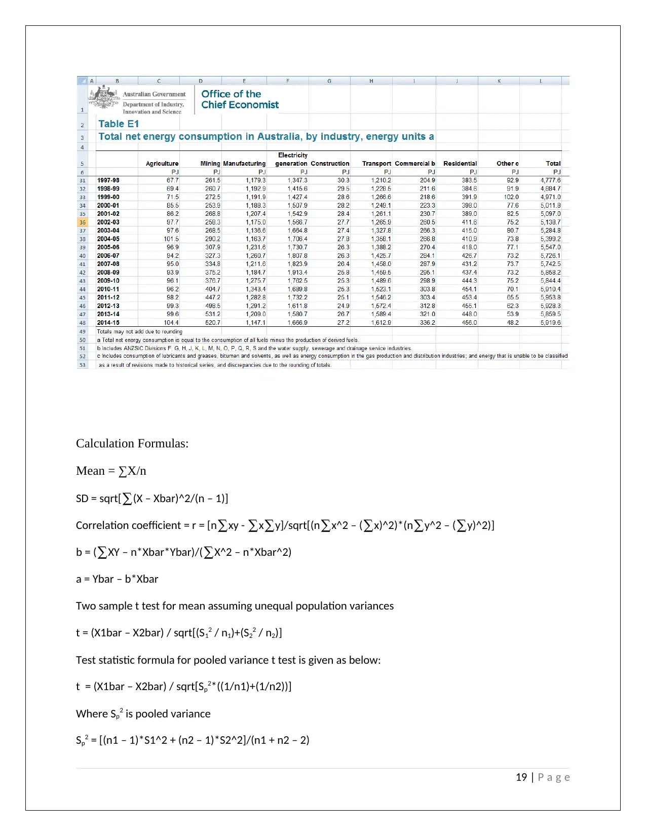
Calculation Formulas:
Mean = ∑X/n
SD = sqrt[∑(X – Xbar)^2/(n – 1)]
Correlation coefficient = r = [n∑xy - ∑x∑y]/sqrt[(n∑x^2 – (∑x)^2)*(n∑y^2 – (∑y)^2)]
b = (∑XY – n*Xbar*Ybar)/(∑X^2 – n*Xbar^2)
a = Ybar – b*Xbar
Two sample t test for mean assuming unequal population variances
t = (X1bar – X2bar) / sqrt[(S12 / n1)+(S22 / n2)]
Test statistic formula for pooled variance t test is given as below:
t = (X1bar – X2bar) / sqrt[Sp2*((1/n1)+(1/n2))]
Where Sp2 is pooled variance
Sp2 = [(n1 – 1)*S1^2 + (n2 – 1)*S2^2]/(n1 + n2 – 2)
19 | P a g e
Paraphrase This Document
Need a fresh take? Get an instant paraphrase of this document with our AI Paraphraser
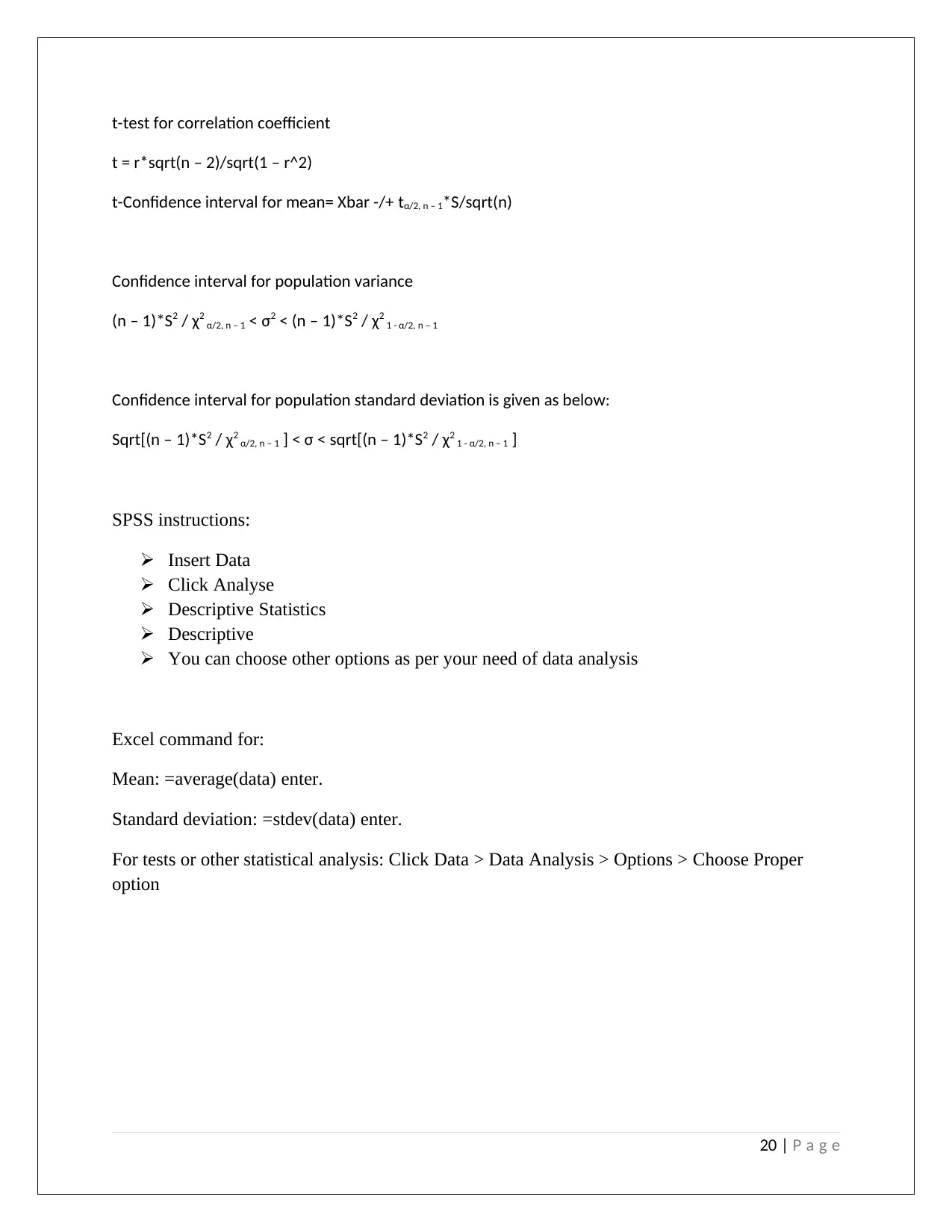
t-test for correlation coefficient
t = r*sqrt(n – 2)/sqrt(1 – r^2)
t-Confidence interval for mean= Xbar -/+ tα/2, n – 1*S/sqrt(n)
Confidence interval for population variance
(n – 1)*S2 / χ2 α/2, n – 1 < σ2 < (n – 1)*S2 / χ2 1 - α/2, n – 1
Confidence interval for population standard deviation is given as below:
Sqrt[(n – 1)*S2 / χ2 α/2, n – 1 ] < σ < sqrt[(n – 1)*S2 / χ2 1 - α/2, n – 1 ]
SPSS instructions:
Insert Data
Click Analyse
Descriptive Statistics
Descriptive
You can choose other options as per your need of data analysis
Excel command for:
Mean: =average(data) enter.
Standard deviation: =stdev(data) enter.
For tests or other statistical analysis: Click Data > Data Analysis > Options > Choose Proper
option
20 | P a g e
1 out of 20
Related Documents


Your All-in-One AI-Powered Toolkit for Academic Success.
+13062052269
info@desklib.com
Available 24*7 on WhatsApp / Email
![[object Object]](/_next/static/media/star-bottom.7253800d.svg)
Unlock your academic potential
© 2024 | Zucol Services PVT LTD | All rights reserved.