Engineering Maths and Modelling
Added on 2023-04-20
50 Pages9794 Words479 Views
ENGINEERING MATHS AND MODELLING
2
ENGINEERING MATHS AND MODELLING
Executive summary
Matlab is a useful tool for solving complex equations easily. Governing equation of the spring-
mass system is derived by the help of analytical method for the single and double spring-mass
system. It follows Hook's law and Newton's law of motion. Spring mass system follows a
harmonic motion which is also dependable on various factors. The variables on which
displacement is dependent on are mass, spring constant, initial conditions, stiffness, damping
factor, and many others. The effect of those on displacement is shown by the help of graphs and
plotting. Symbolic, Analytical, Euler, ODE45 methods are used in solving the governing motion
equations of spring-mass system in this study. Different values of the independent variables are
taken in here for finding proper analysis. The study reflects the use of those equations in
different methods and also shows the different results found in different methods by the use of
Matlab. Findings regarding the entire topic are mentioned clearly in this report which will help to
get a clear idea about the spring-mass-damping system.
3
ENGINEERING MATHS AND MODELLING
Table of Contents
Introduction......................................................................................................................................4
Question 1........................................................................................................................................4
Key findings.................................................................................................................................9
Question 2......................................................................................................................................10
Key findings...............................................................................................................................18
Question 3......................................................................................................................................20
Key findings...............................................................................................................................33
Conclusion.....................................................................................................................................34
Reference List................................................................................................................................35
Appendices....................................................................................................................................38
4
ENGINEERING MATHS AND MODELLING
Introduction
There are many cases where the relation of motion can be shown with respect to time. Spring
mass system is an example of harmonic motion. It follows Hook's law and Newton's law of
motion. Displacement, velocity, and acceleration can be found of any motion by the help of those
laws. In order to get the solution, we need to solve differential equations. In this study, we will
discuss various methods of solving differential equations. Analytical, Euler, ODE45, numerical
methods are used in this study for solving the governing equation of spring damping system.
Matlab helps us in solving any equation correctly and also in a quick process. The processes,
codes, and methods are required in performing a Matlab program. This study will help in
deriving and solving the governing equation for the spring-mass-damping system and also will
help to analyze the key findings during solving by the use of Matlab.
Question 1
a)
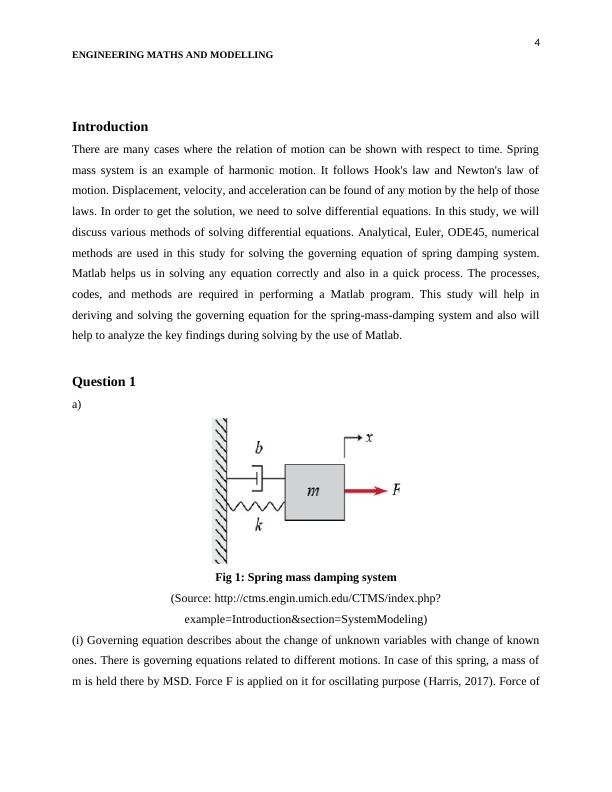
Fig 1: Spring mass damping system
(Source: http://ctms.engin.umich.edu/CTMS/index.php?
example=Introduction§ion=SystemModeling)
(i) Governing equation describes about the change of unknown variables with change of known
ones. There is governing equations related to different motions. In case of this spring, a mass of
m is held there by MSD. Force F is applied on it for oscillating purpose (Harris, 2017). Force of
ENGINEERING MATHS AND MODELLING
Introduction
There are many cases where the relation of motion can be shown with respect to time. Spring
mass system is an example of harmonic motion. It follows Hook's law and Newton's law of
motion. Displacement, velocity, and acceleration can be found of any motion by the help of those
laws. In order to get the solution, we need to solve differential equations. In this study, we will
discuss various methods of solving differential equations. Analytical, Euler, ODE45, numerical
methods are used in this study for solving the governing equation of spring damping system.
Matlab helps us in solving any equation correctly and also in a quick process. The processes,
codes, and methods are required in performing a Matlab program. This study will help in
deriving and solving the governing equation for the spring-mass-damping system and also will
help to analyze the key findings during solving by the use of Matlab.
Question 1
a)
Fig 1: Spring mass damping system
(Source: http://ctms.engin.umich.edu/CTMS/index.php?
example=Introduction§ion=SystemModeling)
(i) Governing equation describes about the change of unknown variables with change of known
ones. There is governing equations related to different motions. In case of this spring, a mass of
m is held there by MSD. Force F is applied on it for oscillating purpose (Harris, 2017). Force of
5
ENGINEERING MATHS AND MODELLING
the damper is given, where b is damping constant. Spring constant k is given there. Deriving a
governing equation, below steps can be used:
F= ma;
a= dx2/dt2;
Considering gravity force, spring force and damping force in this:
mg - k(s+x) = F - b * dx/dt;
mg - k(s+x) = mdx2/dt2 - b * dx/dt;
This is the governing equation for the given figure.
(ii) The conditions here are given for the figure where the governing equation is needed to be
solved. The conditions provided are;
F= 0, m=10 kg, k= 160N/ m, b= 0 N s/m;
x(0) = 0, dx/dt |x=0 = 6;
Gravity force is taken here as negligible. So, force due to gravity is eliminated in the equation.
Besides, spring force is also taken as zero for ease in solution (Cárcamo, Gómez & Fortuny,
2016).
mdx2/dt2 + kx= 0;
dx2/dt2 + (k/m)x = 0;
dx2/dt2 + (160/10)x = 0;
dx2/dt2 + 16x = 0;
Taking the ODE for solution:
D2+ 16= 0;
D= ± 4;
Appendix 1: Symbolic form of solution in Matlab
6
ENGINEERING MATHS AND MODELLING
x(t) = c1 cost 4t + c2 sin 4t;
As, x(0) = 0;
0 = c1 cost 0 + c2 sin 0 = c1 ;
So, x(t) = c2 sin 4t;
x’(t) = 4c2 cos 4t;
As, dx/dt |x=0 = 6, 4c2 = 6
c2 = 3/2= 1.5;
So, x(t) = 1.5 sin 4t;
This is the solution for governing equation in this case.
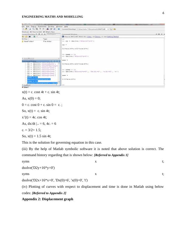
(iii) By the help of Matlab symbolic software it is noted that above solution is correct. The
command history regarding that is shown below: [Referred to Appendix 1]
syms x t;
dsolve('D2y+16*y=0')
syms x t;
dsolve('D2x+16*x=0', 'Dx(0)=6', 'x(0)=0', 't')
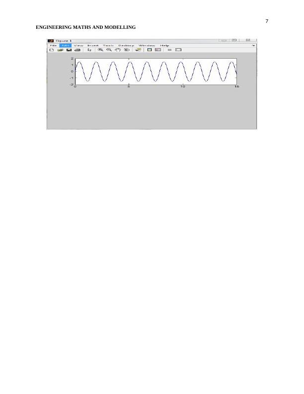
(iv) Plotting of curves with respect to displacement and time is done in Matlab using below
codes: [Referred to Appendix 2]
Appendix 2: Displacement graph
ENGINEERING MATHS AND MODELLING
x(t) = c1 cost 4t + c2 sin 4t;
As, x(0) = 0;
0 = c1 cost 0 + c2 sin 0 = c1 ;
So, x(t) = c2 sin 4t;
x’(t) = 4c2 cos 4t;
As, dx/dt |x=0 = 6, 4c2 = 6
c2 = 3/2= 1.5;
So, x(t) = 1.5 sin 4t;
This is the solution for governing equation in this case.
(iii) By the help of Matlab symbolic software it is noted that above solution is correct. The
command history regarding that is shown below: [Referred to Appendix 1]
syms x t;
dsolve('D2y+16*y=0')
syms x t;
dsolve('D2x+16*x=0', 'Dx(0)=6', 'x(0)=0', 't')
(iv) Plotting of curves with respect to displacement and time is done in Matlab using below
codes: [Referred to Appendix 2]
Appendix 2: Displacement graph
7
ENGINEERING MATHS AND MODELLING
ENGINEERING MATHS AND MODELLING
8
ENGINEERING MATHS AND MODELLING
clear all;
>> close all;
>> t= 0:0.01:15;
>> x= 1.5*sin(4*t);
>> subplot(2,1,1);
>> plot(t,x);
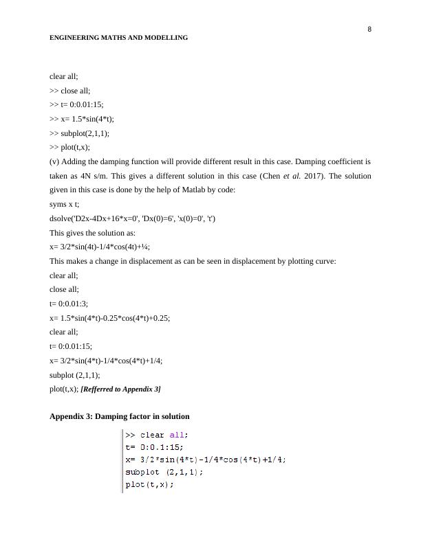
(v) Adding the damping function will provide different result in this case. Damping coefficient is
taken as 4N s/m. This gives a different solution in this case (Chen et al. 2017). The solution
given in this case is done by the help of Matlab by code:
syms x t;
dsolve('D2x-4Dx+16*x=0', 'Dx(0)=6', 'x(0)=0', 't')
This gives the solution as:
x= 3/2*sin(4t)-1/4*cos(4t)+¼;
This makes a change in displacement as can be seen in displacement by plotting curve:
clear all;
close all;
t= 0:0.01:3;
x= 1.5*sin(4*t)-0.25*cos(4*t)+0.25;
clear all;
t= 0:0.01:15;
x= 3/2*sin(4*t)-1/4*cos(4*t)+1/4;
subplot (2,1,1);
plot(t,x); [Refferred to Appendix 3]
Appendix 3: Damping factor in solution
ENGINEERING MATHS AND MODELLING
clear all;
>> close all;
>> t= 0:0.01:15;
>> x= 1.5*sin(4*t);
>> subplot(2,1,1);
>> plot(t,x);
(v) Adding the damping function will provide different result in this case. Damping coefficient is
taken as 4N s/m. This gives a different solution in this case (Chen et al. 2017). The solution
given in this case is done by the help of Matlab by code:
syms x t;
dsolve('D2x-4Dx+16*x=0', 'Dx(0)=6', 'x(0)=0', 't')
This gives the solution as:
x= 3/2*sin(4t)-1/4*cos(4t)+¼;
This makes a change in displacement as can be seen in displacement by plotting curve:
clear all;
close all;
t= 0:0.01:3;
x= 1.5*sin(4*t)-0.25*cos(4*t)+0.25;
clear all;
t= 0:0.01:15;
x= 3/2*sin(4*t)-1/4*cos(4*t)+1/4;
subplot (2,1,1);
plot(t,x); [Refferred to Appendix 3]
Appendix 3: Damping factor in solution
End of preview
Want to access all the pages? Upload your documents or become a member.
Related Documents
Force-Transient Response of 1DOF System with Numerical Convolution, Laplace Transform and MATLABlg...
|19
|5903
|331
Hydrodynamic force on a square cylinderlg...
|22
|3371
|89
Numerical Method for Simple Initial Value Problemlg...
|28
|3455
|38
Effect of KC and damping coefficient on power extraction in a cylinderlg...
|30
|3481
|44
Simple Initial Value Problemlg...
|31
|3578
|22
Effect of KC Number and Damping Coefficient on Power Extraction in a Circular Cylinderlg...
|29
|3620
|33