Force-Transient Response of 1DOF System with Numerical Convolution, Laplace Transform and MATLAB
Added on 2023-06-11
19 Pages5903 Words331 Views
1 Introduction (5 points)
In this particular assignment the objective is to create a force-transient response of a 1
Degree of freedom system which is excited by an aperiodic input force. Then the
response of the system is solved using Numerical convolution, Laplace transform
method and software solution using MATLAB. In MATLAB dsolve and ode45 function is
used to solve the differential equation of the system in time domain. The system is a
mass-spring and damper system with specific parameters as described in the later
section. The solution of the system is obtained in graphical form via plots in MATLAB
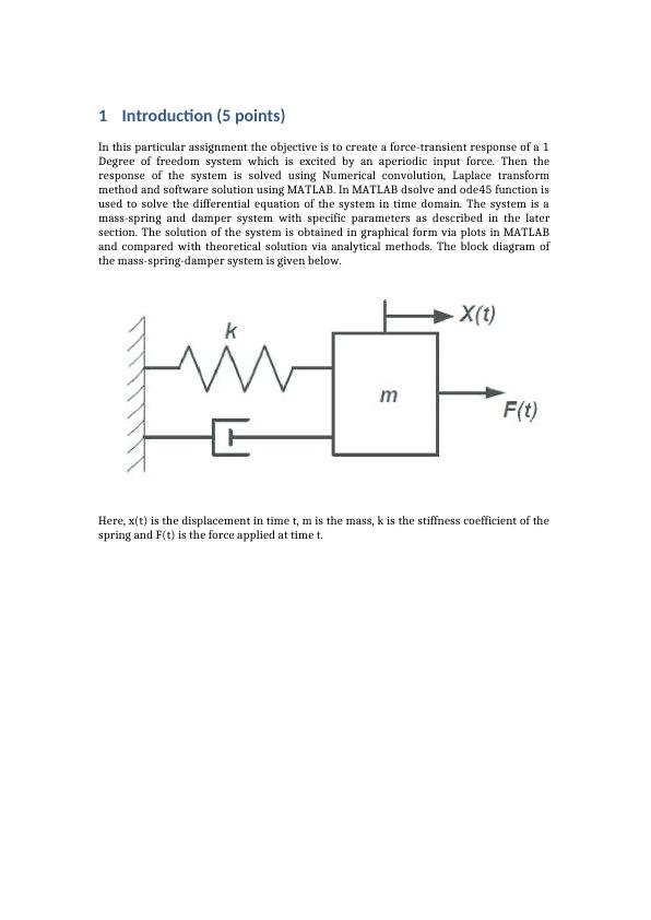
and compared with theoretical solution via analytical methods. The block diagram of
the mass-spring-damper system is given below.
Here, x(t) is the displacement in time t, m is the mass, k is the stiffness coefficient of the
spring and F(t) is the force applied at time t.
In this particular assignment the objective is to create a force-transient response of a 1
Degree of freedom system which is excited by an aperiodic input force. Then the
response of the system is solved using Numerical convolution, Laplace transform
method and software solution using MATLAB. In MATLAB dsolve and ode45 function is
used to solve the differential equation of the system in time domain. The system is a
mass-spring and damper system with specific parameters as described in the later
section. The solution of the system is obtained in graphical form via plots in MATLAB
and compared with theoretical solution via analytical methods. The block diagram of
the mass-spring-damper system is given below.
Here, x(t) is the displacement in time t, m is the mass, k is the stiffness coefficient of the
spring and F(t) is the force applied at time t.
Technical characteristics of 1DOF system (5 points)
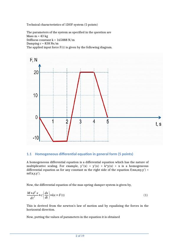
The parameters of the system as specified in the question are
Mass m = 43 kg
Stiffness constant k = 165888 N/m
Damping c = 838 Ns/m
The applied input force F(t) is given by the following diagram.
1.1 Homogeneous differential equation in general form (5 points)
A homogeneous differential equation is a differential equation which has the nature of
multiplicative scaling. For example, y’’(x) = y’(x) + k*y(x) + x is a homogeneous
differential equation as for any constant m the right side of the equation f(mx,my,y’) =
mf(x,y,y’).
Now, the differential equation of the mas-spring-damper system is given by,
M∗d2 x
d t2 +c ( dx
dt ) +kx =F(t) (1)
This is derived from the newton’s law of motion and by equalizing the forces in the
horizontal direction.
Now, putting the values of parameters in the equation it is obtained
2 of 19
43∗d2 x
d t2 +838 ( dx
dt )+165888 x=F(t)
1.2 Find natural frequency, damping ratio and damped frequency if
applicable (5 points)
The natural frequency (wn), damping ratio ( ) and damped frequency (wd) is obtainedζ
by the following method. The natural frequency is the frequency at which the system
tends to oscillate when any of the damping or driving force is absent. The damping ratio
is a dimensionless measure through which the decay of the oscillatory behaviour is
represented after some disturbance has occurred.
Rearranging the equation (1) we get
m ( d2 x
d t2 )=F ( t ) – kx – c∗( dx
dt ) (1)
Now, dividing both sides by k we get
m
k ( d2 x
d t2 )= F ( t )
k – x – c
k ∗( dx
dt )
Hence, the natural frequency of the system is
wn = √ k
m= √ 165888
43 =62.1117 rad /sec, damping ratio ( ) =ζ 838
2∗√ 165888∗43 = 0.1569
The damped frequency wd=62.1117∗√ 1−0.15692 = 61.3424 rad/sec.
1.3 Define transfer function (5 points)
The transfer function of a system is the ratio of output and input. This is basically a
mathematical function that relates the output of the device to its input. It is also
represented as a graph where the independent scalar input is plotted against the
dependent scalar output. The graph is also known as characteristics curve or the
transfer curve. The transfer function is often represented in s domain.
Now, for obtaining the transfer function of the above system Laplace transform is taken
on both sides of equation (1) assuming the initial conditions as zero.
m s2 X (s )=F ( s ) – k∗X ( s ) – c∗s∗X ( s )
Hence,
X ( s ) ( m s2+ cs+ k )=F ( s ) => X ( s )
F ( s ) = 1
ms2 +cs +k
3 of 19
Now, putting the values of the parameters
X ( s )
F ( s ) = 1
ms2 +cs +k = 1
43 s2 +838 s +165888
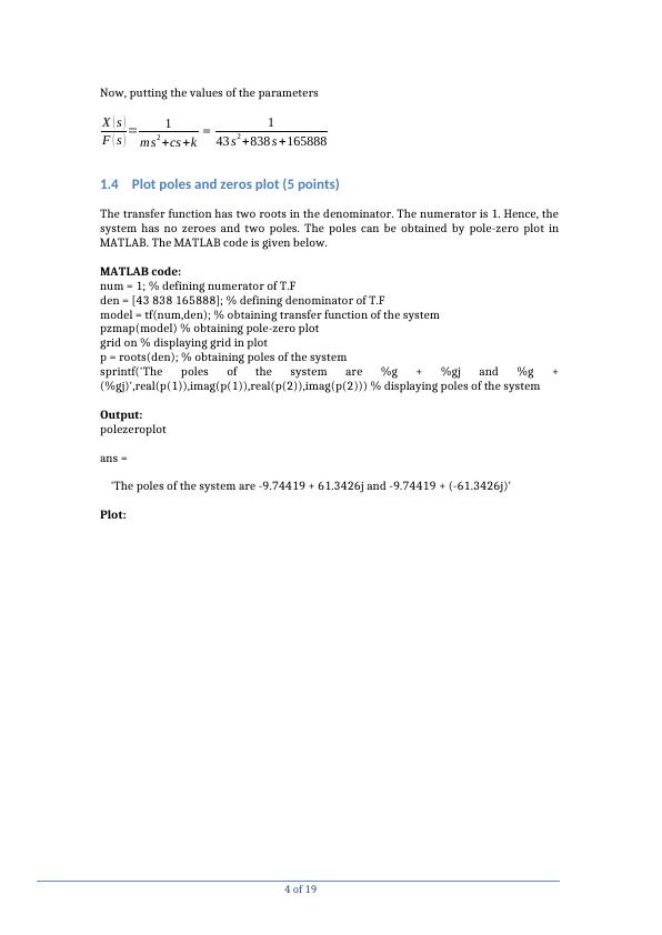
1.4 Plot poles and zeros plot (5 points)
The transfer function has two roots in the denominator. The numerator is 1. Hence, the
system has no zeroes and two poles. The poles can be obtained by pole-zero plot in
MATLAB. The MATLAB code is given below.
MATLAB code:
num = 1; % defining numerator of T.F
den = [43 838 165888]; % defining denominator of T.F
model = tf(num,den); % obtaining transfer function of the system
pzmap(model) % obtaining pole-zero plot
grid on % displaying grid in plot
p = roots(den); % obtaining poles of the system
sprintf('The poles of the system are %g + %gj and %g +
(%gj)',real(p(1)),imag(p(1)),real(p(2)),imag(p(2))) % displaying poles of the system
Output:
polezeroplot
ans =
'The poles of the system are -9.74419 + 61.3426j and -9.74419 + (-61.3426j)'
Plot:
4 of 19
X ( s )
F ( s ) = 1
ms2 +cs +k = 1
43 s2 +838 s +165888
1.4 Plot poles and zeros plot (5 points)
The transfer function has two roots in the denominator. The numerator is 1. Hence, the
system has no zeroes and two poles. The poles can be obtained by pole-zero plot in
MATLAB. The MATLAB code is given below.
MATLAB code:
num = 1; % defining numerator of T.F
den = [43 838 165888]; % defining denominator of T.F
model = tf(num,den); % obtaining transfer function of the system
pzmap(model) % obtaining pole-zero plot
grid on % displaying grid in plot
p = roots(den); % obtaining poles of the system
sprintf('The poles of the system are %g + %gj and %g +
(%gj)',real(p(1)),imag(p(1)),real(p(2)),imag(p(2))) % displaying poles of the system
Output:
polezeroplot
ans =
'The poles of the system are -9.74419 + 61.3426j and -9.74419 + (-61.3426j)'
Plot:
4 of 19
End of preview
Want to access all the pages? Upload your documents or become a member.
Related Documents
ENS6160: Signals & Systemslg...
|12
|720
|276
Engineering Maths and Modellinglg...
|50
|9794
|479
Vehicle Suspension System Analysis Assignment | Deskliblg...
|10
|1655
|429
Mathematical Analysis of Vehicle Suspension Systemlg...
|11
|1362
|168
Effect of KC and damping coefficient on power extraction in a cylinderlg...
|30
|3481
|44
Numerical Method for Simple Initial Value Problemlg...
|28
|3455
|38