Understanding State Space Representation

This assignment delves into the concept of state space representation used in modeling dynamic systems. It defines state variables as the minimum set required to describe a system's behavior and introduces state-space equations for both continuous-time and discrete-time systems. The document differentiates between time-varying and time-invariant systems, highlighting how the state-space equations are modified accordingly. Furthermore, it discusses the advantages of using state space representations and provides examples illustrating their application.

ENS6160: SIGNAL AND SYSTEM
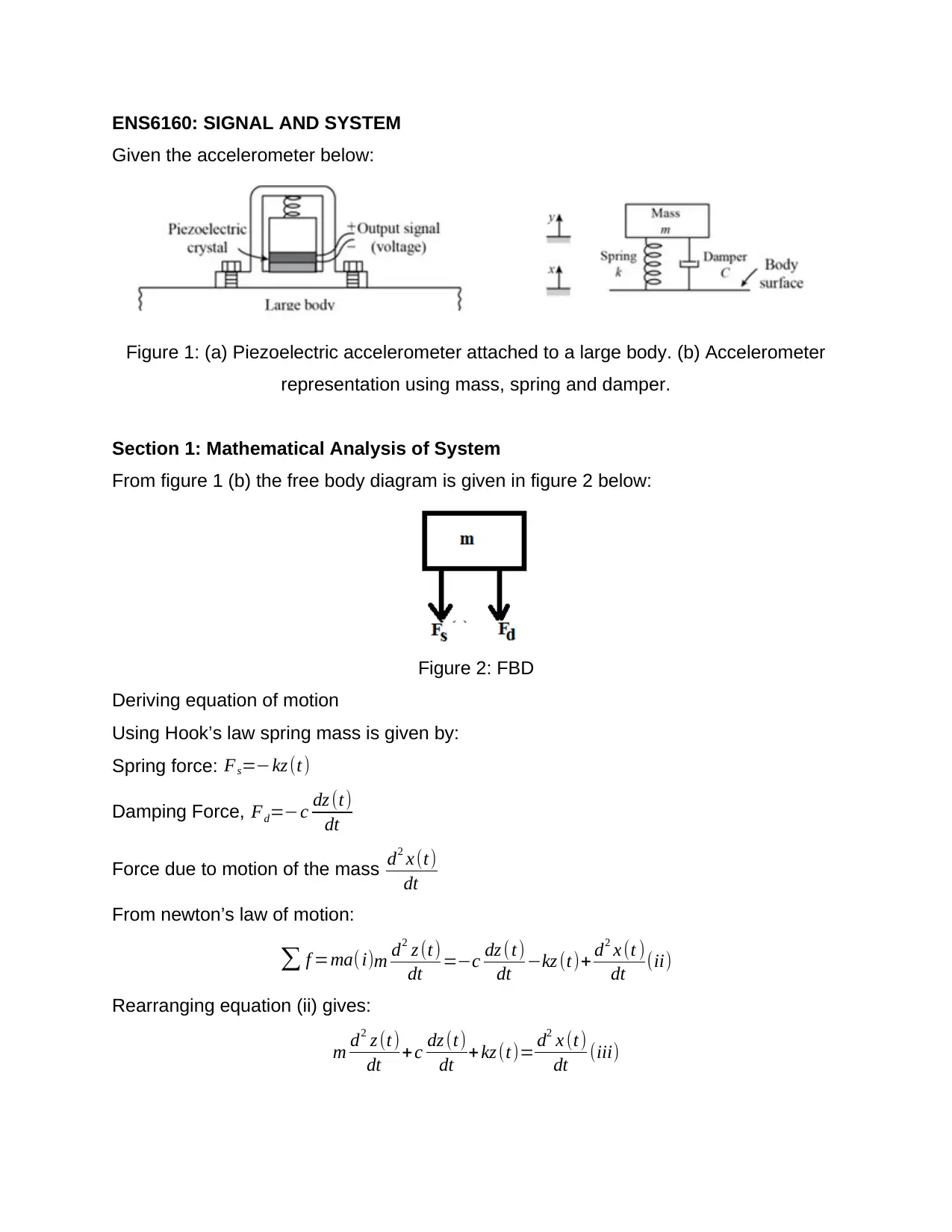
Given the accelerometer below:
Figure 1: (a) Piezoelectric accelerometer attached to a large body. (b) Accelerometer
representation using mass, spring and damper.
Section 1: Mathematical Analysis of System
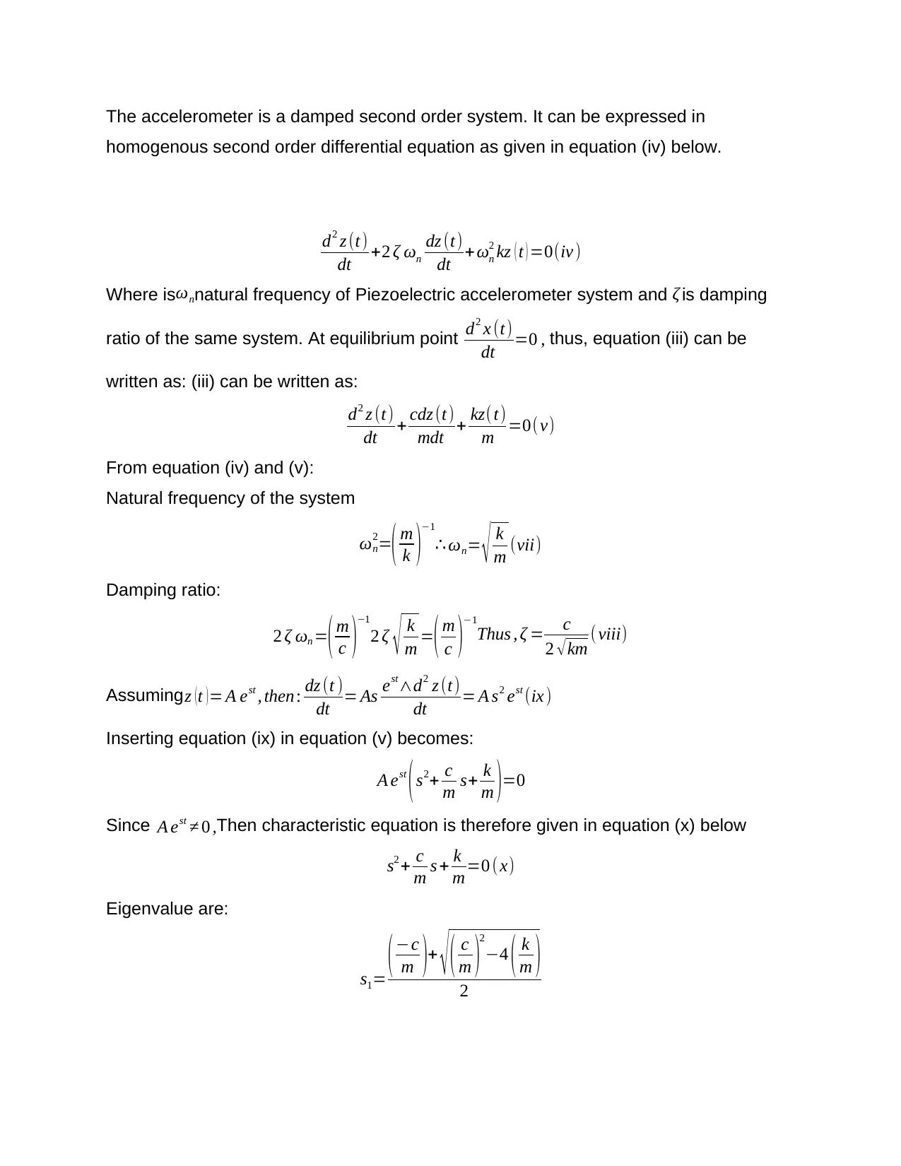
From figure 1 (b) the free body diagram is given in figure 2 below:
Figure 2: FBD
Deriving equation of motion
Using Hook’s law spring mass is given by:
Spring force: Fs=−kz(t )
Damping Force, Fd=−c dz (t)
dt
Force due to motion of the mass d2 x (t)
dt
From newton’s law of motion:
∑ f =ma(i)m d2 z (t)
dt =−c dz (t)
dt −kz (t)+ d2 x (t )
dt (ii)
Rearranging equation (ii) gives:
m d2 z (t)
dt +c dz (t)
dt + kz (t)= d2 x (t)
dt (iii)

The accelerometer is a damped second order system. It can be expressed in
homogenous second order differential equation as given in equation (iv) below.
d2 z (t)
dt +2 ζ ωn
dz (t)
dt +ωn
2 kz ( t ) =0(iv)
Where is ωnnatural frequency of Piezoelectric accelerometer system and ζ is damping
ratio of the same system. At equilibrium point d2 x (t)
dt =0 , thus, equation (iii) can be
written as: (iii) can be written as:
d2 z (t)
dt + cdz (t)
mdt + kz(t)
m =0(v)
From equation (iv) and (v):
Natural frequency of the system
ωn
2=( m
k )
−1
∴ ωn= √ k
m (vii)
Damping ratio:
2 ζ ωn =( m
c )
−1
2 ζ √ k
m =( m
c )
−1
Thus , ζ = c
2 √km ( viii)
Assuming z ( t ) = A est , then : dz (t )
dt = As est∧d2 z (t)
dt = A s2 est (ix)
Inserting equation (ix) in equation (v) becomes:
A est
(s2+ c
m s+ k
m )=0
Since A est ≠ 0 ,Then characteristic equation is therefore given in equation (x) below
s2 + c
m s + k
m=0 (x)
Eigenvalue are:
s1= ( −c
m )+ √ ( c
m )
2
−4 ( k
m )
2

s2= (−c
m )− √ ( c
m )2
−4 ( k
m )
2
From equation (x);
i) if 0<ζ <1 the Piezoelectric accelerometer is underdamped: here, the system
oscillates with a frequency equal to ωd=ωn √ 1−ζ2
ii) if ζ =1the Piezoelectric accelerometer is critically damped: here, the
Piezoelectric accelerometer slowly returns to equilibrium
iii) if ζ 1 ,the Piezoelectric accelerometer is over-damped: here, The Piezoelectric
accelerometer returns to equilibrium faster
Taking m=4.3 ×106 kg :k =508 N /m
From equation (vii), the natural frequency of accelerometer is:
ωn= √ k
m= √ 508
4.3 ×10−6 =10869.20121rad / s
Taking ζ =1 ,then from equation (viii):
ζ = c
2 √ km ⟹ c=2 ζ √ km=2 √ 4.3 ×106 ×508=0.09347513038 kg/ s
Section 2: System analysis using MATLAB.
For ζ =1
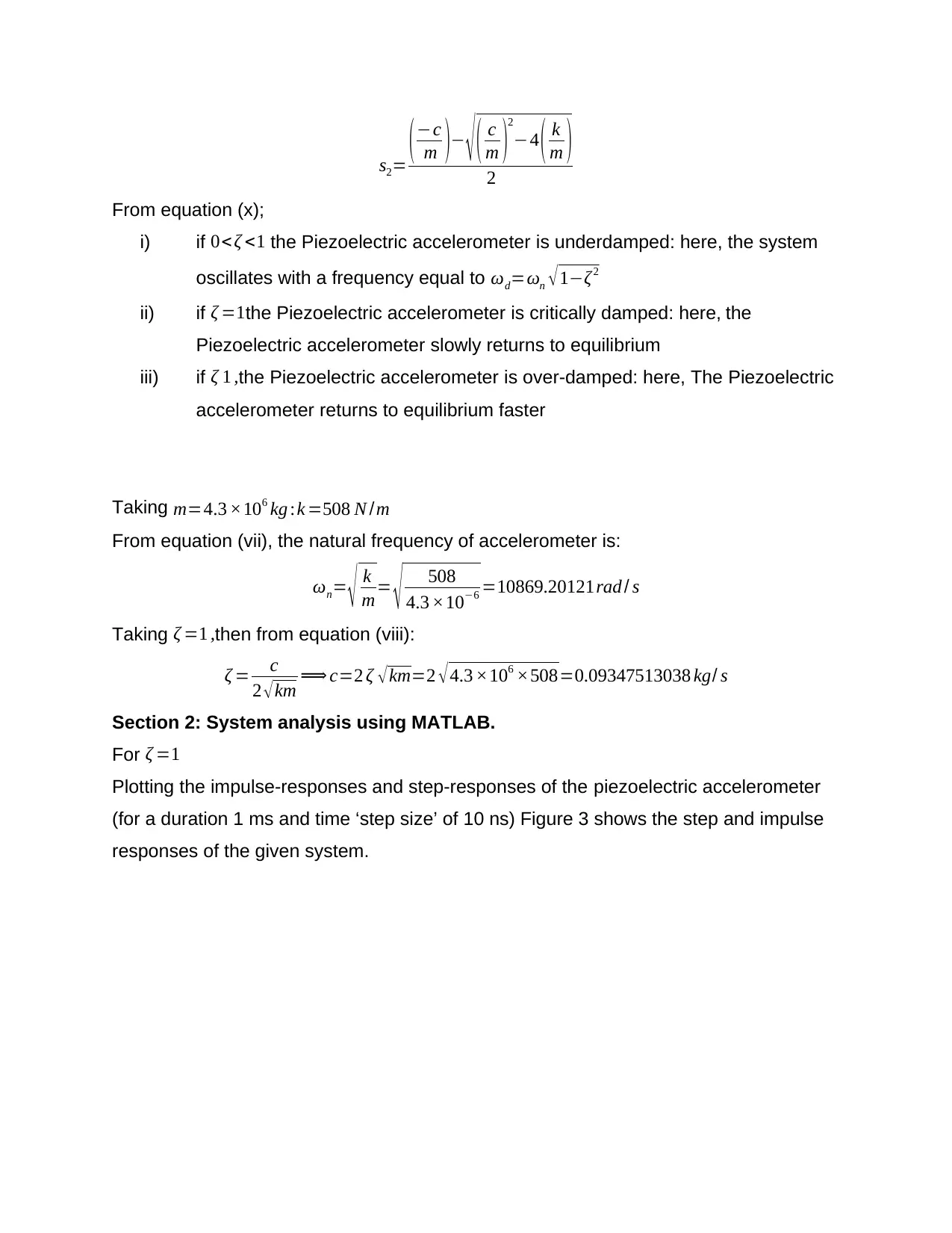
Plotting the impulse-responses and step-responses of the piezoelectric accelerometer
(for a duration 1 ms and time ‘step size’ of 10 ns) Figure 3 shows the step and impulse
responses of the given system.

0 0.1 0.2 0.3 0.4 0.5 0.6 0.7 0.8 0.9 1
10-3
0
1
2
3
4 10-5 Impulse Response
Time (seconds)
Amplitude
0 0.1 0.2 0.3 0.4 0.5 0.6 0.7 0.8 0.9 1
10-3
0
0.5
1 10-8 Step Response
Time (seconds)
Amplitude
Figure 3: The impulse and step responses of the given system
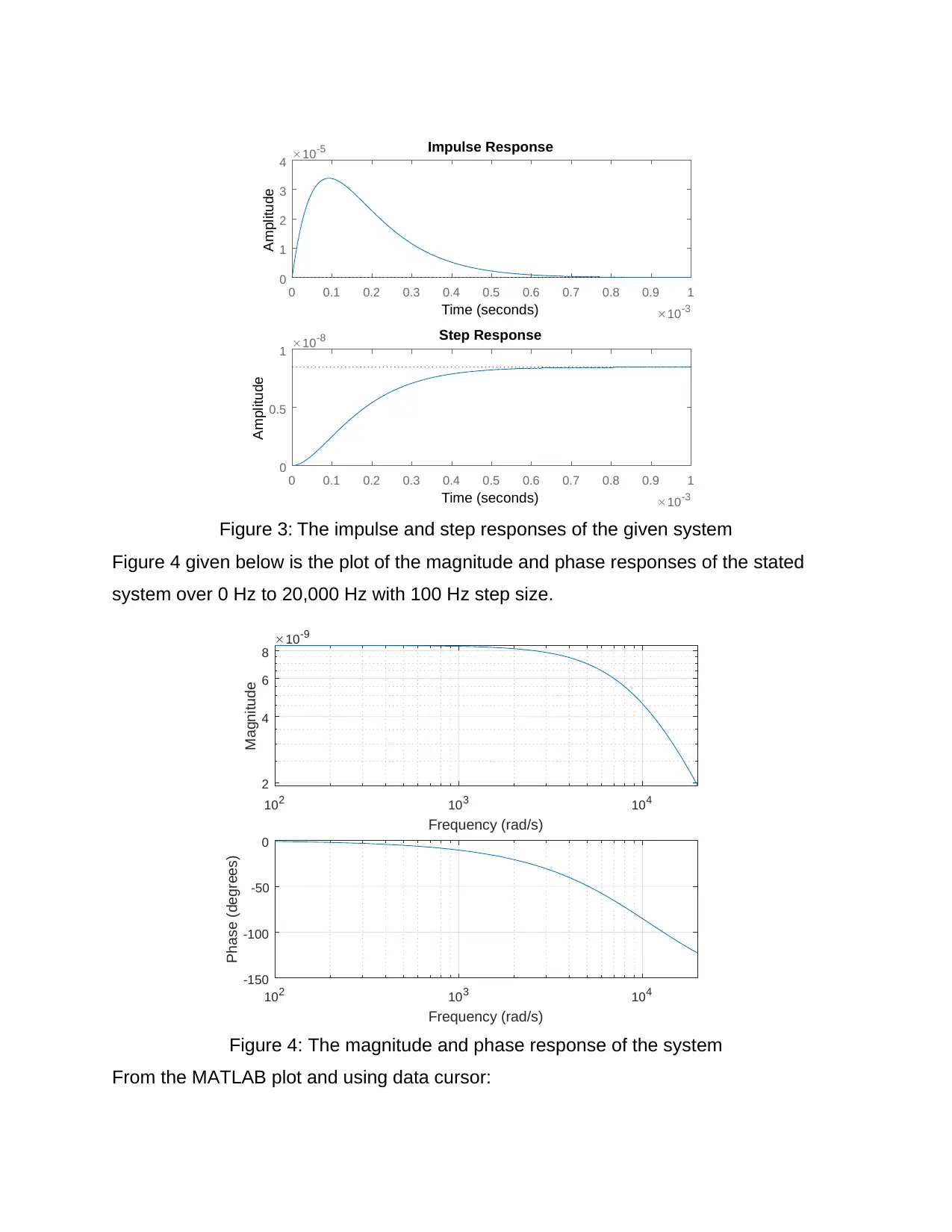
Figure 4 given below is the plot of the magnitude and phase responses of the stated
system over 0 Hz to 20,000 Hz with 100 Hz step size.
102 103 104
Frequency (rad/s)
-150
-100
-50
0
Phase (degrees)
102 103 104
Frequency (rad/s)
2
4
6
8
Magnitude
10-9
Figure 4: The magnitude and phase response of the system
From the MATLAB plot and using data cursor:

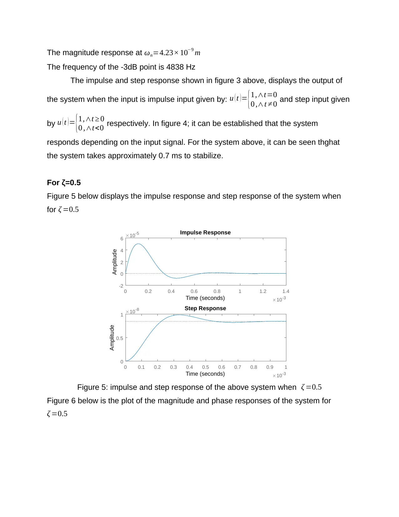
The magnitude response at ωn=4.23× 10−9 m
The frequency of the -3dB point is 4838 Hz
The impulse and step response shown in figure 3 above, displays the output of
the system when the input is impulse input given by: u ( t ) = {1,∧t=0
0 ,∧t ≠ 0 and step input given
by u ( t ) = {1,∧t ≥ 0
0 ,∧t<0 respectively. In figure 4; it can be established that the system
responds depending on the input signal. For the system above, it can be seen thghat
the system takes approximately 0.7 ms to stabilize.
For ζ=0.5
Figure 5 below displays the impulse response and step response of the system when
for ζ =0.5
0 0.2 0.4 0.6 0.8 1 1.2 1.4
10-3
-2
0
2
4
6 10-5 Impulse Response
Time (seconds)
Amplitude
0 0.1 0.2 0.3 0.4 0.5 0.6 0.7 0.8 0.9 1
10-3
0
0.5
1 10-8 Step Response
Time (seconds)
Amplitude
Figure 5: impulse and step response of the above system when ζ =0.5
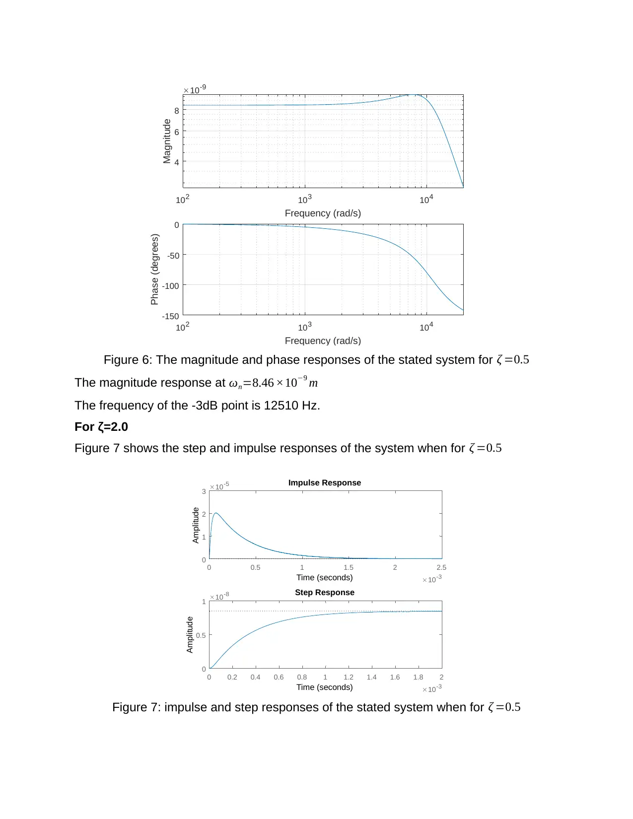
Figure 6 below is the plot of the magnitude and phase responses of the system for
ζ =0.5

102 103 104
Frequency (rad/s)
-150
-100
-50
0
Phase (degrees)
102 103 104
Frequency (rad/s)
4
6
8
Magnitude
10-9
Figure 6: The magnitude and phase responses of the stated system for ζ =0.5
The magnitude response at ωn=8.46 ×10−9 m
The frequency of the -3dB point is 12510 Hz.
For ζ=2.0
Figure 7 shows the step and impulse responses of the system when for ζ =0.5
0 0.5 1 1.5 2 2.5
10-3
0
1
2
3 10-5 Impulse Response
Time (seconds)
Amplitude
0 0.2 0.4 0.6 0.8 1 1.2 1.4 1.6 1.8 2
10-3
0
0.5
1 10-8 Step Response
Time (seconds)
Amplitude
Figure 7: impulse and step responses of the stated system when for ζ =0.5

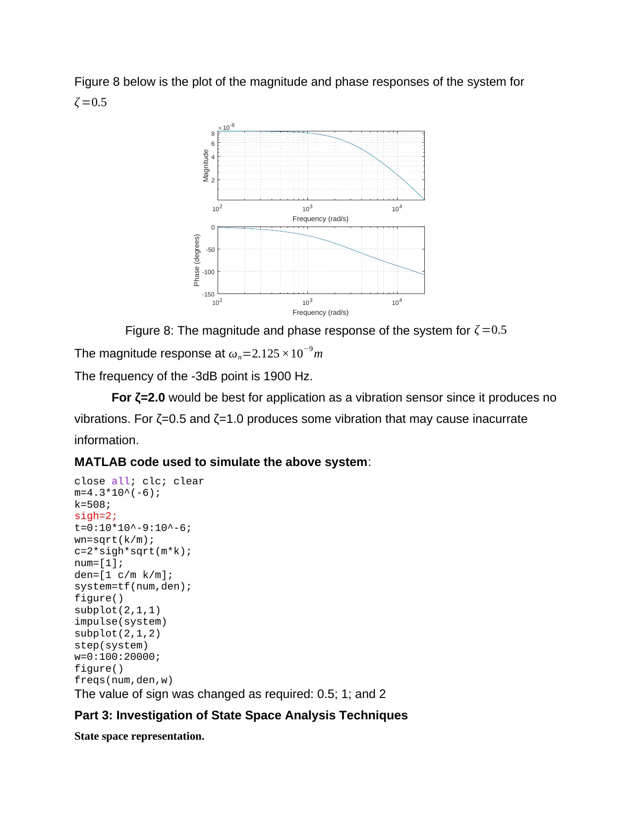
Figure 8 below is the plot of the magnitude and phase responses of the system for
ζ =0.5
102 103 104
Frequency (rad/s)
-150
-100
-50
0
Phase (degrees)
102 103 104
Frequency (rad/s)
2
4
6
8
Magnitude
10-9
Figure 8: The magnitude and phase response of the system for ζ =0.5
The magnitude response at ωn=2.125 ×10−9 m
The frequency of the -3dB point is 1900 Hz.
For ζ=2.0 would be best for application as a vibration sensor since it produces no
vibrations. For ζ=0.5 and ζ=1.0 produces some vibration that may cause inacurrate
information.
MATLAB code used to simulate the above system:
close all; clc; clear
m=4.3*10^(-6);
k=508;
sigh=2;
t=0:10*10^-9:10^-6;
wn=sqrt(k/m);
c=2*sigh*sqrt(m*k);
num=[1];
den=[1 c/m k/m];
system=tf(num,den);
figure()
subplot(2,1,1)
impulse(system)
subplot(2,1,2)
step(system)
w=0:100:20000;
figure()
freqs(num,den,w)
The value of sign was changed as required: 0.5; 1; and 2
Part 3: Investigation of State Space Analysis Techniques
State space representation.

A current control systems are very complex since some of them have numerous inputs same as to
the outputs, and they are interconnected in convoluted way. In the process of analyzing these kind of
systems, it is important reducing the involvedness of the mathematical expressions that arises in these
system. Furthermore, reduction of computer for tiresome computation required in the analyzing of such
system. The method of state-space analysis of the system is better suitable for these kind of computations.
Although conventional control theories are based on transfer function or the inputs–outputs
relationship, current control theorems are based on the descriptions of systems equations in form of n-
ODE (order differential equation), where it can be united or convolved into a 1st order vector matrixes
differential equations. Using vector-matrix notations prominently make the mathematical representations
of system of equations simpler. When the number of state variable increases, the numeral of outputs, or
the inputs has no impact on the complexity of systems’ equation. Indeed, the analysis of such
sophisticated MIMO (multi-input multi-output) systems can be done through techniques which are more
slightly complicated as compared to those needed for systems analysis of 1st-order scalar differential
equation.
Definition of valuables.
State
The state of the dynamic systems are the lowest sets of variables (referred to as state variables) in
such a way that awareness of those variable at time t1=t0 (initial time), in cooperation with the awareness
of inputs for timet1=t0, entirely controls the behaviors of systems for any given time t1 ≥ t0 It can be
noted that the concepts of states are by no mean limited to physical system only. It is also applicable to
social systems, economic systems, biological systems, and other system.
State Vector.
If n_state variables are required to entirely define the behaviors of any stated systems, then these
n_state variables might be reflected in the nth component of a vector_X. Such vectors are referred to as a
state vector. State vectors are therefore vectors that defines uniquely the systems state x (t) for any time
t1 ≥ t0 at the state at t1=t0 are specified and the inputs u(t ) for t1 ≥ t 0 is given.
State Space.
The nth_dimensional space whose coordinates axes comprises the
x1 axis , x2 axis, x3 axis …… … … … … . xn axis, wherever x1 , x2 , x3 ,… … xn are state variables, is
referred to as a state space. At all state vectors might be characterized by a point in the state space.
State Variables.

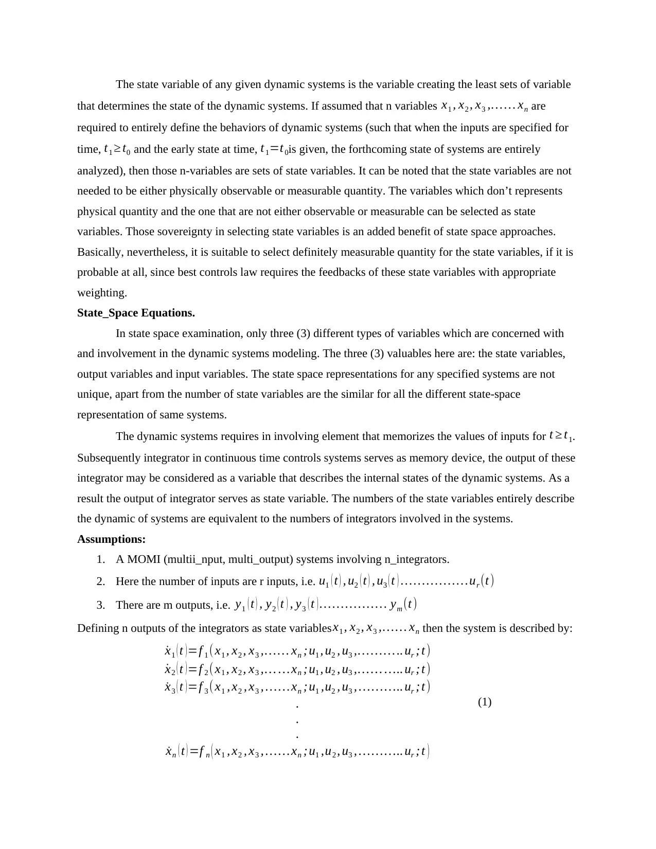
The state variable of any given dynamic systems is the variable creating the least sets of variable
that determines the state of the dynamic systems. If assumed that n variables x1 , x2 , x3 ,… … xn are
required to entirely define the behaviors of dynamic systems (such that when the inputs are specified for
time, t1 ≥ t0 and the early state at time, t1=t0is given, the forthcoming state of systems are entirely
analyzed), then those n-variables are sets of state variables. It can be noted that the state variables are not
needed to be either physically observable or measurable quantity. The variables which don’t represents
physical quantity and the one that are not either observable or measurable can be selected as state
variables. Those sovereignty in selecting state variables is an added benefit of state space approaches.
Basically, nevertheless, it is suitable to select definitely measurable quantity for the state variables, if it is
probable at all, since best controls law requires the feedbacks of these state variables with appropriate
weighting.
State_Space Equations.
In state space examination, only three (3) different types of variables which are concerned with
and involvement in the dynamic systems modeling. The three (3) valuables here are: the state variables,
output variables and input variables. The state space representations for any specified systems are not
unique, apart from the number of state variables are the similar for all the different state-space
representation of same systems.
The dynamic systems requires in involving element that memorizes the values of inputs for t ≥ t1.
Subsequently integrator in continuous time controls systems serves as memory device, the output of these
integrator may be considered as a variable that describes the internal states of the dynamic systems. As a
result the output of integrator serves as state variable. The numbers of the state variables entirely describe
the dynamic of systems are equivalent to the numbers of integrators involved in the systems.
Assumptions:
1. A MOMI (multii_nput, multi_output) systems involving n_integrators.
2. Here the number of inputs are r inputs, i.e. u1 ( t ) , u2 ( t ) , u3 ( t ) … … … … … .ur (t )
3. There are m outputs, i.e. y1 ( t ) , y2 ( t ) , y3 ( t ) … … … … … . ym (t )
Defining n outputs of the integrators as state variables x1 , x2 , x3 ,… … xn then the system is described by:
˙x1 ( t ) =f 1 (x1 , x2 , x3 ,… … xn ;u1 , u2 , u3 ,… … ….. ur ; t)
˙x2 ( t ) =f 2 (x1 , x2 , x3 ,… … xn ;u1 , u2 , u3 ,… … ….. ur ; t)
˙x3 ( t ) =f 3 (x1 , x2 , x3 , … … xn ;u1 ,u2 , u3 , … … ….. ur ; t)
.
.
.
˙xn ( t ) =f n ( x1 , x2 , x3 , … … xn ;u1 ,u2 , u3 , … … ….. ur ; t )
(1)

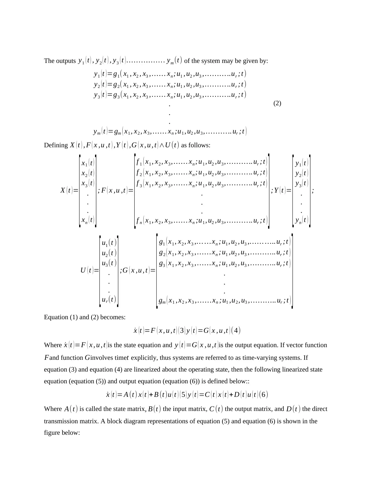
The outputs y1 ( t ) , y2 ( t ) , y3 ( t ) … … … … … . ym (t) of the system may be given by:
y1 ( t ) =g1( x1 , x2 , x3 , … … xn ;u1 , u2 ,u3 , … …… ..ur ; t)
y2 ( t ) =g2( x1 , x2 , x3 , … … xn ;u1 , u2 ,u3 , … …… ..ur ; t)
y3 ( t ) =g3 ( x1 , x2 , x3 , … … xn ;u1 , u2 ,u3 , … …… ..ur ; t)
.
.
.
ym ( t ) =gm ( x1 , x2 , x3 , … … xn ;u1 , u2 ,u3 , … … ….. ur ;t )
(2)
Defining X ( t ) , F ( x ,u ,t ) ,Y ( t ) ,G ( x , u , t ) ∧U (t) as follows:
X ( t ) =
[ x1 ( t )
x2 ( t )
x3 ( t )
.
.
.
xn ( t )
] ; F ( x ,u ,t ) =
[ f 1 ( x1 , x2 , x3 , … … xn ;u1 , u2 ,u3 , … … … .. ur ; t )
f 2 ( x1 , x2 , x3 , … … xn ;u1 , u2 ,u3 , … … … .. ur ; t )
f 3 ( x1 , x2 , x3 , … … xn ;u1 , u2 ,u3 , … … … .. ur ; t )
.
.
.
f n ( x1 , x2 , x3 , … … xn ;u1 , u2 ,u3 , … … … .. ur ; t )
] ; Y ( t ) =
[ y1 ( t )
y2 ( t )
y3 ( t )
.
.
.
yn ( t )
] ;
U ( t ) =
[ u1 (t )
u2 (t )
u3 (t )
.
.
.
ur (t)
] ;G ( x ,u , t ) =
[ g1 ( x1 , x2 , x3 ,… … xn ; u1 , u2 , u3 ,… … ….. ur ;t )
g2 ( x1 , x2 , x3 , … … xn ; u1 ,u2 , u3 , … … ….. ur ;t )
g3 ( x1 , x2 , x3 , … … xn ; u1 ,u2 , u3 , … … ….. ur ;t )
.
.
.
gm ( x1 , x2 , x3 , … … xn ;u1 ,u2 , u3 , … … ….. ur ; t )
]Equation (1) and (2) becomes:
˙x (t )=F ( x , u , t ) ( 3 ) y ( t ) =G ( x , u ,t ) ( 4)
Where ˙x (t )=F ( x , u , t )is the state equation and y ( t ) =G ( x , u ,t )is the output equation. If vector function
Fand function Ginvolves timet explicitly, thus systems are referred to as time-varying systems. If
equation (3) and equation (4) are linearized about the operating state, then the following linearized state
equation (equation (5)) and output equation (equation (6)) is defined below::
˙x (t )= A (t) x ( t )+ B (t )u ( t ) ( 5 ) y ( t ) =C ( t ) x ( t ) +D ( t ) u ( t ) (6)
Where A(t) is called the state matrix, B(t) the input matrix, C (t) the output matrix, and D(t ) the direct
transmission matrix. A block diagram representations of equation (5) and equation (6) is shown in the
figure below:

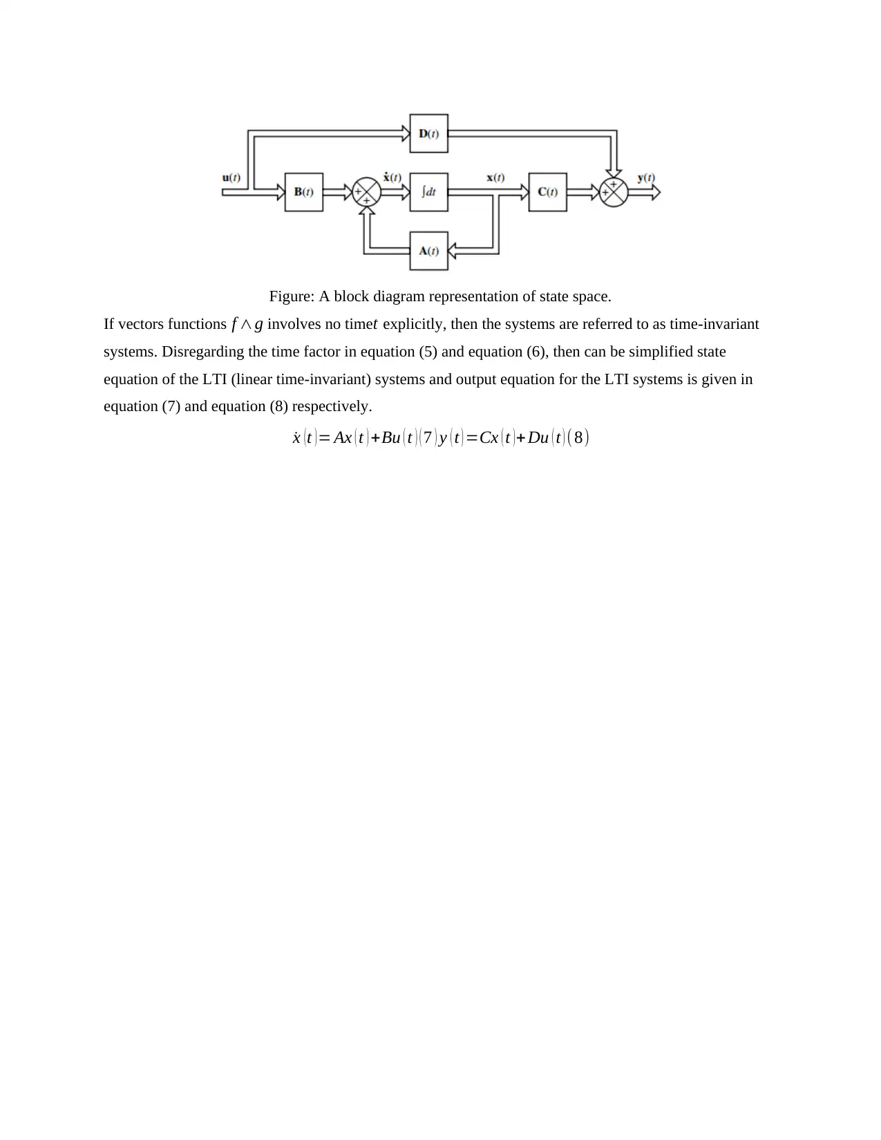
Figure: A block diagram representation of state space.
If vectors functions f ∧g involves no timet explicitly, then the systems are referred to as time-invariant
systems. Disregarding the time factor in equation (5) and equation (6), then can be simplified state
equation of the LTI (linear time-invariant) systems and output equation for the LTI systems is given in
equation (7) and equation (8) respectively.
˙x (t )= Ax ( t ) +Bu ( t ) ( 7 ) y ( t ) =Cx ( t )+ Du ( t ) (8)