Temperature Evolution in 1D Heat Conduction

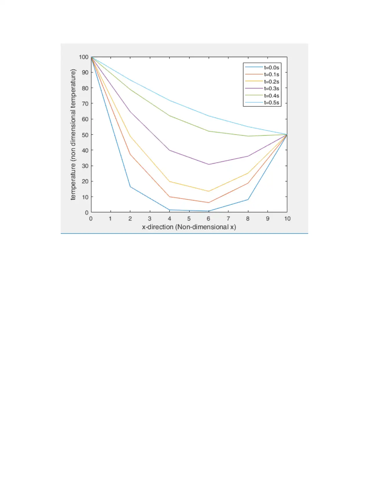
This assignment involves simulating the behavior of temperature in a one-dimensional heat conduction scenario. The provided data outlines time steps and corresponding non-dimensional temperatures at various points along the length (x) of the system. Students are tasked with plotting these temperature distributions for several time steps to visualize how the temperature evolves over time. The analysis requires understanding and interpreting the non-dimensional temperature profiles.

FACULTY OF ENGINEERING AND INFORMATION SCIENCES
UNIVERSITY OF WOLLONGONG
ENGG952 ENGINEERING COMPUTING
SPRING SESSION – 2017
GROUP OR INDIVIDUAL DETAILS
NAMES OF MEMBERS
REGISTRATION NUMBERS
DATE OF SUBMISSION

ASSIGNMENT 2
QUESTION 1 (50%)
Mass-Spring-Damper system for an Ordinary Differential Equation
Free vibrations in a mechanical system are caused by initial conditions of the parameters:
displacement, velocity, or acceleration where no external force is allowed to interact. The
mechanical system in the free vibration will oscillate with its natural frequency and eventually
settle down to zero as a result of damping effects.
∑ f =ma
m d2 x
d t2 +c ( dx
dt )+kx =0
Dividing through by mass, m,
d2 x
d t2 + c
m ( dx
dt )+ k
m x=0
The natural frequency of the system and the damping ratio are replaced as shown in
the following equation,
d2 x
d t2 + 2ζ w0 ( dx
dt )+w0
2 x=0
Where,
w0= √ k
m , ζ = c
2 √ km
The solution to the differential equation.
λ1,2=−2 ζ ω0 ± √ 4 ζ2 ω0
2 −4 ω0
2
2
Therefore,
λ1,2=−ζ ω0 ± ω0 √ ζ 2−1
The transient solution of the system is given as,
xt =A e
(−ζ ω0 +ω0 √ζ 2−1 ) t +B e
( −ζ ω0 −ω0 √ζ 2−1 ) t
The constants A and B are obtained when the initial conditions are inserted. The final
solution is obtained as,
From the initial conditions,
w0=1 , ζ=0.125
xt =A e
(−0.125+ ω0 √ζ 2−1 ) t + B e
(−ζ ω0−ω0 √ζ 2−1 ) t
The Runge-Kutta Heun Method considering a certain range or period of time

tspan=[0:0.1:50];
y0=[0.02;0];
[t,y]=ode45('unforced2',tspan,y0);
plot(t,y(:,1));
grid on
xlabel('time')
ylabel('Displacement')
title('Critically-damped Modelling of MSD system (C=40)')
%% order 647236
tspan=[0:0.1:50];
y0=[0.02;0];
[t,y]=ode45('unforced1',tspan,y0);
plot(t,y(:,1));
grid on
xlabel('time')
ylabel('Displacement')
title('Under-damped Modelling of MSD system (C=5)')
hold on;
%% order 647236
function yp=unforced2(t,y)
c=40;
m=20;
k=20;
yp= [y(2); (-((c/m)*y(2))-((k/m)*y(1)))];
%% order 647236
function yp=unforced1(t,y)
c=5;
m=20;
k=20;
yp= [y(2); (-((c/m)*y(2))-((k/m)*y(1)))];
The graphical illustration of the behavior of the mass-spring-damper for an under-damped and
critically-damped system are shown in the same axes. The critically damped reduces to zero
faster than the under-damped. The damping coefficient determines the rate at which the signal
reduces its amplitude or magnitude as it travels.

QUESTION 2 (50%)
Transient heat conduction in an insulated rod. The non-dimensional form is expressed as
Solution

The explicit finite difference method and the implicit crank-Nicholson method are used to solve
this equation. The explicit method of parabolic PDE is simple to program though governed by a
criterion for the solution to converge. The steps used are restricted by the criterion. There are
implicit methods employed as well as they are more stable. There are two implicit method
namely the simple implicit method and the Crank-Nicholson method which are simple with low
accuracy and complex with high accuracy respectively. The explicit schemes are conditionally
stable for the parabolic partial differential equations. The case study is on heat conduction
equation over time variable with one spatial dimension.
(i) Implicit method
The elliptic parabolic PDEs can be solved using the finite Difference Method. The
dimension of time in this case is open and the initial condition is set at t=0.
Step 1: the temperature for the next time step is calculated and indexed as shown
below,
For the ith node: -
Space domain at time l: ∂2 T
∂ x2 =(T ¿¿ i+1l−2 Ti
l +T i−1
l )/ ∆ x2 ¿
Time domain at node i: ∂T
∂ t = Ti
l +1−T i
l
∆ t
The time derivative, unfortunately, is less accurate than the spatial derivative. The
central difference in terms of x, indexed by I,
α ( Ti +1
l −2 Ti
l +T i−1
l
∆ x2 )= Ti
l +1−T i
l
∆ t
λ= α Δ t
Δ x2
¿
T i
l+1=T i
l + λ(Ti +1
l −2T i
l +T i−1
l )
¿

T i
l+1= λT i−1
l + ( 1−2 λ ) T i
l+ λ Ti +1
l
where the time stepl+1∧time stepl are used .
To ensure stability the time step is limited by a space interval such that,
( 1−2 λ ) ≥ 0 , λ ≤1 /2
(ii) Crank-Nicholson method
Clear all; % clear memory of variables and figures
clc;
close all;
alfa = 0.835;
x0 = 0; % starting x
xm = 10; % ending x
t0 = 0; % starting t
tn = 0.5; % ending t
m = 5; % number of interval in x direction
n = 300; % number of interval in t direction
x = linspace(x0,xm,m+1); % x coordinates of the nodes
t = linspace(t0,tn,n+1); % t coordinates of the nodes
del_x = (xm - x0)/m; % delta x
del_t = (tn - t0)/n; % delta t
hh = del_x*del_x; % constant
r = hh/del_t; % constant
p = 2*r/alfa; % constant
%%%%% Setting the initial conditions %%%%%%%%%%%%%%%%%%%%%%%%%%%%%%%%
%f = inline('sin(x)'); % initial condition expression
T(1,1:m+1) = 0; % set T at t = 0
%%%%% Setting the boundary conditions %%%%%%%%%%%%%%%%%%%%%%%%%%%%%%%%
T(2:n+1,1) = 100.0; % T at x = x0
T(2:n+1,m+1) = 50.0; % T at x = xm
%%%%% Setting the matrix form and solve them at each time step
A_left(1:m-1,1:m-1) = 0;
A_right(1:m-1,1:m-1) = 0;
for i = 1:m-1
A_left(i,i) = -2 - p;
A_right(i,i) = 2 - p;
if i < m-1;
A_left(i,i+1) = 1;
A_right(i,i+1) = -1;
end
if i > 1;
A_left(i,i-1) = 1;
A_right(i,i-1) = -1;
end
end
for j = 1:n
b = A_right*T(j,2:m)';
b(1) = b(1) - T(j,1) - T(j+1,1);

b(m-1) = b(m-1) - T(j,m+1) - T(j+1,m+1);
T(j+1,2:m) = A_left\b;
end
%this figure is only suitalbe for dt=0.1sec only.
figure(1)
x=x0:del_x:xm
plot(x,T(11,:),x,T(31,:), x,T(51,:), x,T(101,:),x,T(201,:),x,T(301,:))
legend('t=0.0s','t=0.1s','t=0.2s','t=0.3s','t=0.4s','t=0.5s');
xlabel('x-direction (Non-dimensional x)'); ylabel('temperature (non
dimensional temperature)');
To calculate the temperatures for the first step seeks to move from the known to the unknown,
Node 1 Node 2 Node 3 Node 4 Node 5 Node 6
x=0 x=2 x=4 x=6 x=8 x=10
time step
0 t=0.0 100 0 0 0 0 50
time step
1 t=0.1 100 2.0875 0 0 1.04375 50
time step
2 t=0.2 100
4.08784
7
0.04357
7
0.02178
8
2.04392
3 50
time step
3 t=0.3 100
6.00558
9
0.12754
6
0.06445
5
3.00279
4 50
time step
4 t=0.4 100
7.84501
8
0.24893
3 0.12711
3.92252
3 50
time step
5 t=0.5 100
9.61018
5
0.40495
8
0.20888
2
4.80516
1 50
time step
6 t=0.6
time step
7 t=0.7
time step
8 t=0.8
time step
9 t=0.9
time step
10 t=0.10
Plot for the non-dimensional temperature versus the non-dimensional length for a few typical
values of non-dimensional times. They are used to demonstrate the evolution of the temperature
at different times as shown in the table above. The time differs per time step.