Difference Between Security Market Line

FIN201 Assignment, Trimester 1 2018
Investment management
‘

TABLE OF CONTENTS
Introduction................................................................................................................................4
Difference between Security Market Line (SML) and Capital Market Line (CML).................4
Importance of minimum variance portfolio...............................................................................8
Relevancy of CAPM in comparison to other equations...........................................................11
Conclusion................................................................................................................................13
References................................................................................................................................14

LIST OF FIGURES
Figure 1: Capital market line graph...........................................................................................4
Figure 2: Security market line....................................................................................................6
Figure 3: Frontier of Minimum variance portfolio....................................................................8
Figure 4: Capital asset pricing model.......................................................................................10

INTRODUCTION
The present study is based on evaluation advance concepts of investment portfolio
management in order to gain an understanding for making better investment decisions. In the
first part, the study will cover the difference between Security Market Line and Capital
Market Line by considering proper graph and its interpretation. Further, discussion of
minimum variance portfolio and its significance will be done by making use of relevant
examples. In the last part of the study; relevancy of CAPM model will be discussed in
comparison to another model available for computation of return on investment.
DIFFERENCE BETWEEN SECURITY MARKET LINE (SML)
AND CAPITAL MARKET LINE (CML)
The capital market line arises from the integration of free of risk asset and the market
portfolio. Every point together with the CML has premium profiles of risk-return to the
portfolio on the effective edge (Asness, Frazzini and Pedersen, 2012). Derivation of CML is
held by drawing a tangent line from the point of intercept upon the efficient frontier till when
the expected return is equivalent to the free of risk rate of return (Hodnett and Hsieh, 2012).
A line is put in use in the pricing approach of a capital asset to demonstrate the return rates
for the efficient portfolio based on the free of risk rate of return and the risk level, i.e.,
standards deviation for a specified portfolio (Lee and Su, 2014).
The CML is stated to be top-notch to the efficient frontier, as it considers the addition of risk-
free asset within the portfolio (Brown, 2012). The CAPM which stands for capital asset
pricing model illustrates that essentially the market portfolio is the efficient frontier.
Formula: E(Ri) = RF + SDc×{E(RM)-RF}/SDm
In which the SDC refers to a portfolio standard deviation C return, while the SDM is
regarded as a market-return standard deviation.

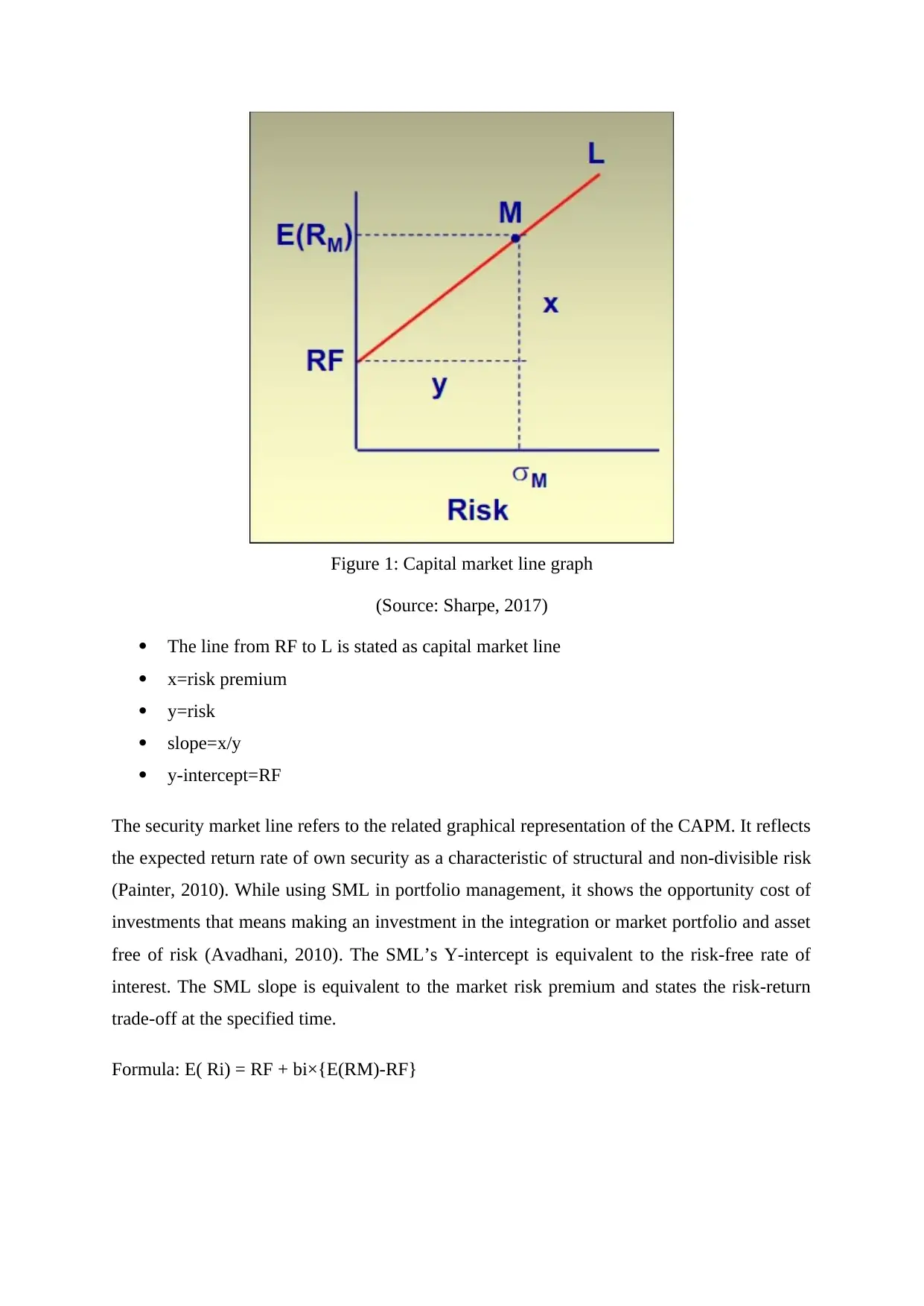
Figure 1: Capital market line graph
(Source: Sharpe, 2017)
 The line from RF to L is stated as capital market line
 x=risk premium
 y=risk
 slope=x/y
 y-intercept=RF
The security market line refers to the related graphical representation of the CAPM. It reflects
the expected return rate of own security as a characteristic of structural and non-divisible risk
(Painter, 2010). While using SML in portfolio management, it shows the opportunity cost of
investments that means making an investment in the integration or market portfolio and asset
free of risk (Avadhani, 2010). The SML’s Y-intercept is equivalent to the risk-free rate of
interest. The SML slope is equivalent to the market risk premium and states the risk-return
trade-off at the specified time.
Formula: E( Ri) = RF + bi×{E(RM)-RF}

In which the E (Ri) is regarded as an expected return of security, the risk-free rate is the RF,
and the beta coefficient of security is abbreviated as bi, and the E (RM) means the expected
market return.
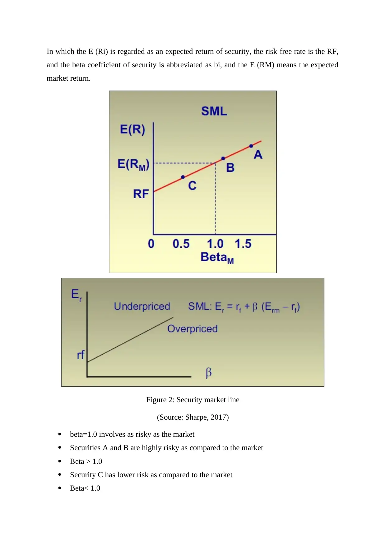
Figure 2: Security market line
(Source: Sharpe, 2017)
 beta=1.0 involves as risky as the market
 Securities A and B are highly risky as compared to the market
 Beta > 1.0
 Security C has lower risk as compared to the market
 Beta< 1.0

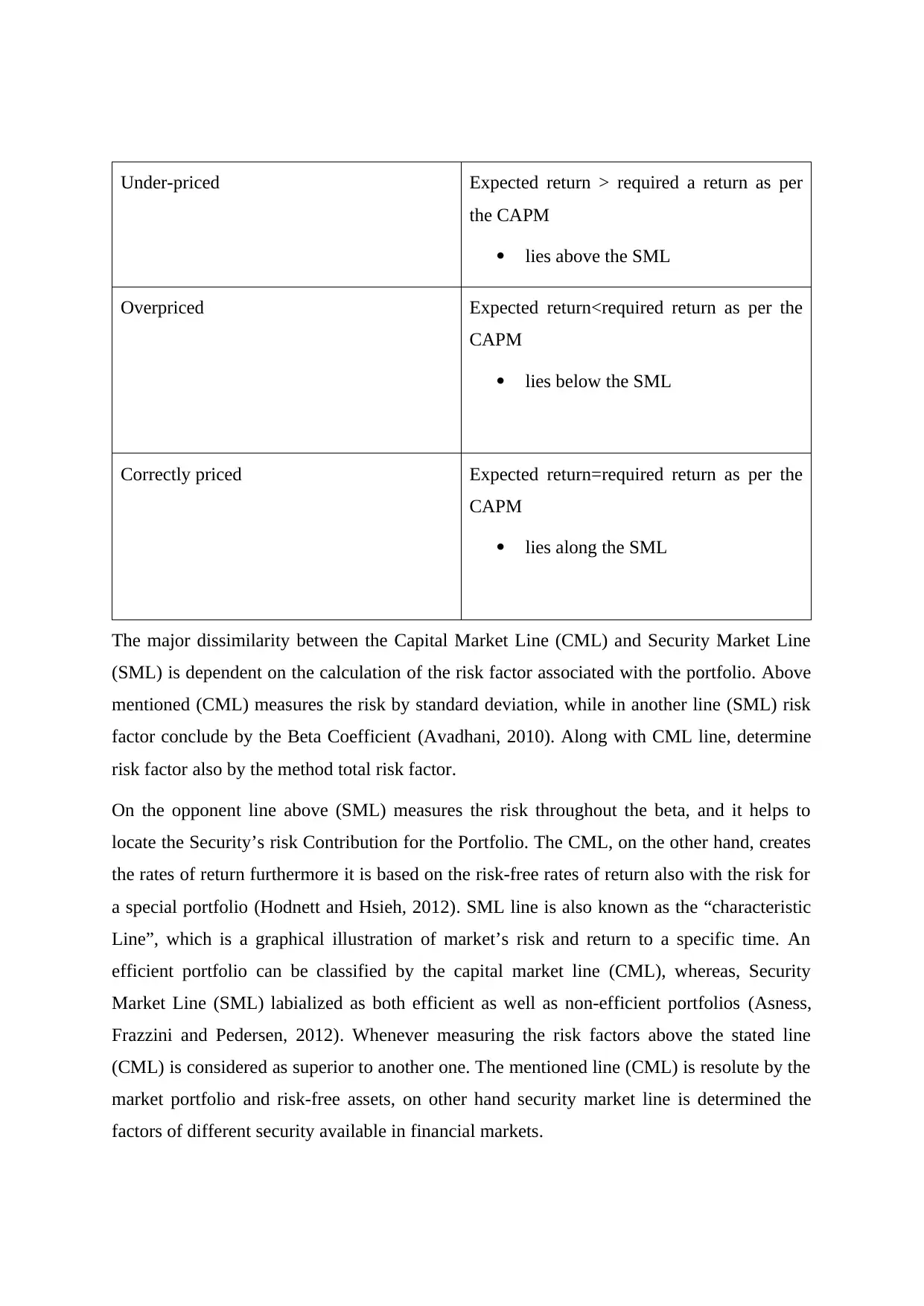
Under-priced Expected return > required a return as per
the CAPM
 lies above the SML
Overpriced Expected return<required return as per the
CAPM
 lies below the SML
Correctly priced Expected return=required return as per the
CAPM
 lies along the SML
The major dissimilarity between the Capital Market Line (CML) and Security Market Line
(SML) is dependent on the calculation of the risk factor associated with the portfolio. Above
mentioned (CML) measures the risk by standard deviation, while in another line (SML) risk
factor conclude by the Beta Coefficient (Avadhani, 2010). Along with CML line, determine
risk factor also by the method total risk factor.
On the opponent line above (SML) measures the risk throughout the beta, and it helps to
locate the Security’s risk Contribution for the Portfolio. The CML, on the other hand, creates
the rates of return furthermore it is based on the risk-free rates of return also with the risk for
a special portfolio (Hodnett and Hsieh, 2012). SML line is also known as the “characteristic
Line”, which is a graphical illustration of market’s risk and return to a specific time. An
efficient portfolio can be classified by the capital market line (CML), whereas, Security
Market Line (SML) labialized as both efficient as well as non-efficient portfolios (Asness,
Frazzini and Pedersen, 2012). Whenever measuring the risk factors above the stated line
(CML) is considered as superior to another one. The mentioned line (CML) is resolute by the
market portfolio and risk-free assets, on other hand security market line is determined the
factors of different security available in financial markets.

The Capital market line illustrates defined effective portfolio, and both effective and non-
effective portfolio is defined by the graph. When the returns are computed, the CML
portfolios expected return is demonstrated on the Y-axis (Antoniou, Doukas and
Subrahmanyam, 2015). On the contrary to this, for SML, the securities return is presented
with the
Y-axis, whereas for CML, The portfolio standard deviation is presented on the X-axis and for
SML, the Beta of security is represented on the X-axis.
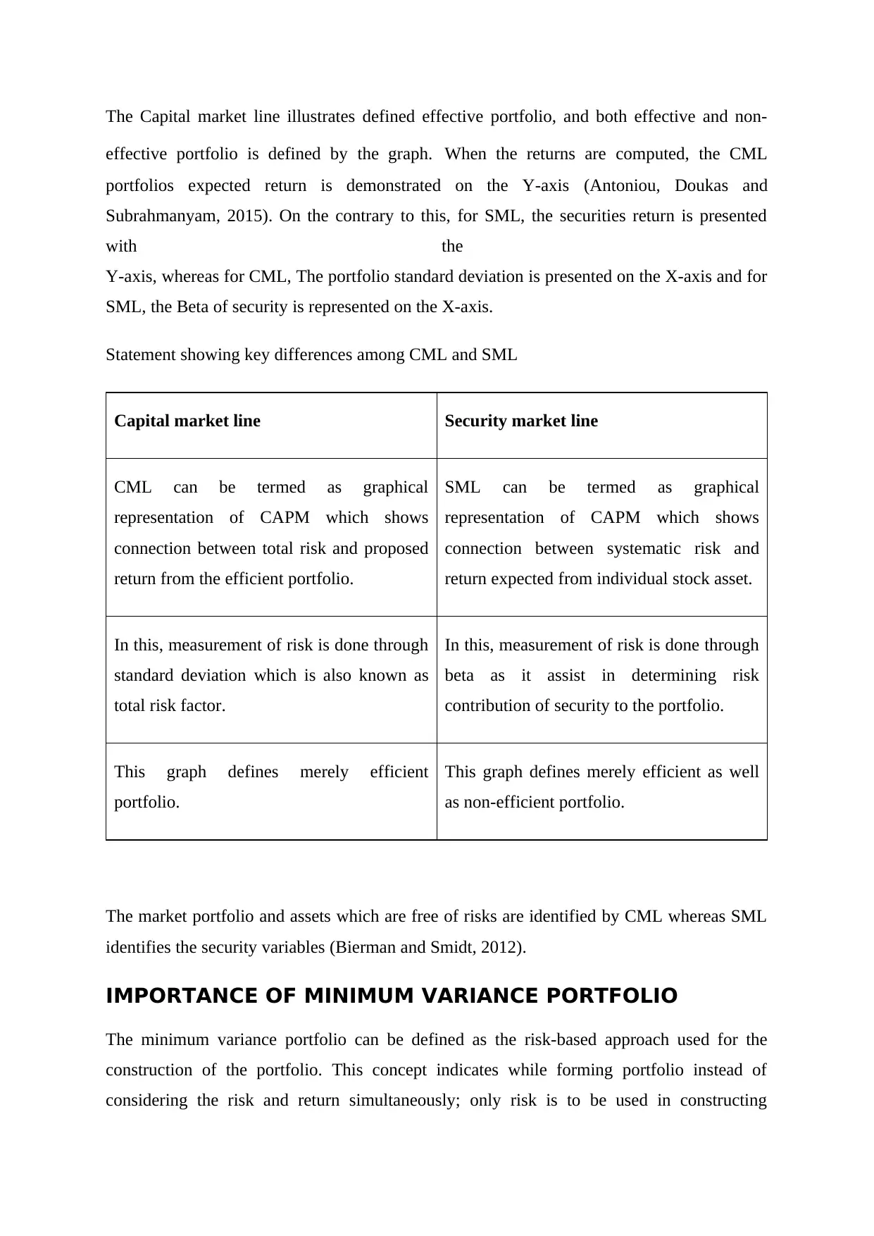
Statement showing key differences among CML and SML
Capital market line Security market line
CML can be termed as graphical
representation of CAPM which shows
connection between total risk and proposed
return from the efficient portfolio.
SML can be termed as graphical
representation of CAPM which shows
connection between systematic risk and
return expected from individual stock asset.
In this, measurement of risk is done through
standard deviation which is also known as
total risk factor.
In this, measurement of risk is done through
beta as it assist in determining risk
contribution of security to the portfolio.
This graph defines merely efficient
portfolio.
This graph defines merely efficient as well
as non-efficient portfolio.
The market portfolio and assets which are free of risks are identified by CML whereas SML
identifies the security variables (Bierman and Smidt, 2012).
IMPORTANCE OF MINIMUM VARIANCE PORTFOLIO
The minimum variance portfolio can be defined as the risk-based approach used for the
construction of the portfolio. This concept indicates while forming portfolio instead of
considering the risk and return simultaneously; only risk is to be used in constructing

portfolio (Bodnar, Parolya and Schmid, 2018). This approach is viable for investors as the
determination of future returns is not an easy task and estimations made are not accurate in all
cases. Consideration of this aspect leads to forming a more robust portfolio that is less
subjected to estimation of risk. Computation of weights can be done by using following
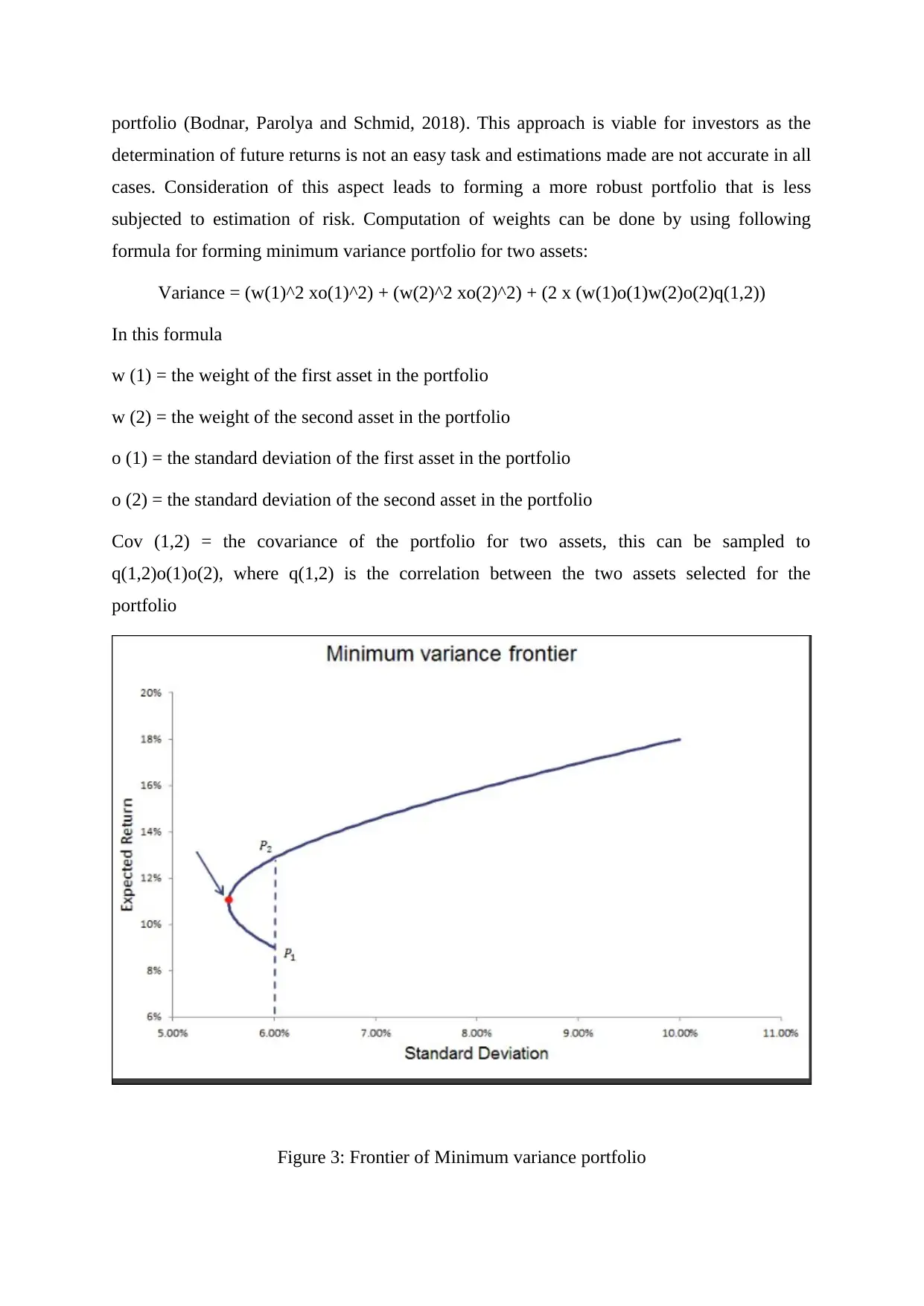
formula for forming minimum variance portfolio for two assets:
Variance = (w(1)^2 xo(1)^2) + (w(2)^2 xo(2)^2) + (2 x (w(1)o(1)w(2)o(2)q(1,2))
In this formula
w (1) = the weight of the first asset in the portfolio
w (2) = the weight of the second asset in the portfolio
o (1) = the standard deviation of the first asset in the portfolio
o (2) = the standard deviation of the second asset in the portfolio
Cov (1,2) = the covariance of the portfolio for two assets, this can be sampled to
q(1,2)o(1)o(2), where q(1,2) is the correlation between the two assets selected for the
portfolio
Figure 3: Frontier of Minimum variance portfolio

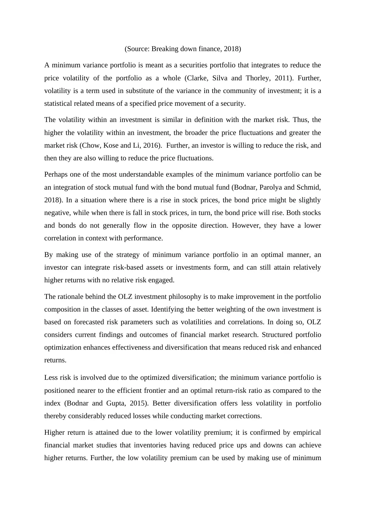
(Source: Breaking down finance, 2018)
A minimum variance portfolio is meant as a securities portfolio that integrates to reduce the
price volatility of the portfolio as a whole (Clarke, Silva and Thorley, 2011). Further,
volatility is a term used in substitute of the variance in the community of investment; it is a
statistical related means of a specified price movement of a security.
The volatility within an investment is similar in definition with the market risk. Thus, the
higher the volatility within an investment, the broader the price fluctuations and greater the
market risk (Chow, Kose and Li, 2016). Further, an investor is willing to reduce the risk, and
then they are also willing to reduce the price fluctuations.
Perhaps one of the most understandable examples of the minimum variance portfolio can be
an integration of stock mutual fund with the bond mutual fund (Bodnar, Parolya and Schmid,
2018). In a situation where there is a rise in stock prices, the bond price might be slightly
negative, while when there is fall in stock prices, in turn, the bond price will rise. Both stocks
and bonds do not generally flow in the opposite direction. However, they have a lower
correlation in context with performance.
By making use of the strategy of minimum variance portfolio in an optimal manner, an
investor can integrate risk-based assets or investments form, and can still attain relatively
higher returns with no relative risk engaged.
The rationale behind the OLZ investment philosophy is to make improvement in the portfolio
composition in the classes of asset. Identifying the better weighting of the own investment is
based on forecasted risk parameters such as volatilities and correlations. In doing so, OLZ
considers current findings and outcomes of financial market research. Structured portfolio
optimization enhances effectiveness and diversification that means reduced risk and enhanced
returns.
Less risk is involved due to the optimized diversification; the minimum variance portfolio is
positioned nearer to the efficient frontier and an optimal return-risk ratio as compared to the
index (Bodnar and Gupta, 2015). Better diversification offers less volatility in portfolio
thereby considerably reduced losses while conducting market corrections.
Higher return is attained due to the lower volatility premium; it is confirmed by empirical
financial market studies that inventories having reduced price ups and downs can achieve
higher returns. Further, the low volatility premium can be used by making use of minimum

variance portfolio in an optimal manner, due to the correlation among own investments are
also considered.
RELEVANCY OF CAPM IN COMPARISON TO OTHER
EQUATIONS
RRR which stands for required rate of return is an element in a lot of metrics implemented in
company finance and valuation of equity. The RRR depicts the requirement of profit in
commencing a project or investment (Fonseca, 2017). Further, RRR could be implemented in
order to aid investors in making a decision if or if not they shall proceed in purchasing
security. On the other hand, company executive and the finance expertise compute the RRR
for investments inclusive of the purchase of possible merger & acquisitions and production-
related equipment’s.
The Capital asset model is regarded as an asset which depicts the connection between
investment risk and expected return in security (Coqueret, 2015). It reflects that the security’s
expected return is equivalent to risk-free return add risk premium, which is done on the basis
of the beta of the same security. The CAMP concept is represented as below:
Figure 4: Capital asset pricing model
(Source: Suntraruk, 2018)

The formula of CAPM is broadly used in the financial sector by several occupations like an
accountant, investment bankers and financial analysts (Fernandez, 2015). It is considered as
an important aspect of the weighted average cost of capital as CAPM helps in calculating the
equity costs.
The formula of CAPM has continued in viable over 40 years of investment analysis due to its
various benefits in comparison to other methods (Coqueret, 2015). One of the major reason,
due to which CAPM is viable that it solely focused on systematic risk while computing rate
of return (Zabarankin, Pavlikov and Uryasev, 2014). This factor indicates the realism that
diversified portfolios fundamentally disregarded all the unsystematic risk stanching from
characteristics of individual asset investment (Fonseca, 2017). This presumption is valid
because; diversification of systematic risk cannot be done, and it is integral to the entire stock
market or to the particular market segment.
WACC is also used immensely in the financial model; it can be implemented to look out for
the NPV and future cash inflows and outflows of the made investment. Additionally, it
computes the entity’s value and ultimately reaches computing equity value (Zabarankin,
Pavlikov and Uryasev, 2014).
CAPM comes with various benefits; it is a calculation which is simple to use that can be
easily tested to gain a variety of potential results for providing confidence with the RRR.
CAPM considers systematic risk, which is apart from other methods, like dividend discount
model. It is also known as market risk and is considered as a significant factor, as it is
unexpected and generally it is not possible to entirely mitigate it as it is not completely
expected. The theory that investors retain a diversified portfolio, same as the market portfolio
makes reduction the unsystematic risk (Suntraruk, 2018). While business lookout for
opportunities, is the mix of business and financial aspects vary from the existing business,
then the other calculations of required return such as the WACC cannot be implemented, but
CAPM can be used (Coqueret, 2015).
CAPM model assists investors to determine the price they should pay for the particular
security by determining its fair price. For example, one stock is comparatively riskier than
other stock; the price of the stock will also fluctuate as per the risk. Same aspects are applied
to the rate of return provided by stock; higher the rate indicates higher market price and vice
versa (Zabarankin, Pavlikov and Uryasev, 2014). Therefore; this model is generally used for
the purpose of determining fair price of investment to be made by the investor. In situation;

where investor determines the return on risk assets, they can apply time value of money to
compute the present value of investment in order to make a viable choice. By extending this
analysis, an investor can compare their fair to market value and can plan for bargain
strategies as per the concerned case of overstatement or understatement.
It can be said that no model is ideal, but every model has its own traits that make them
applicable and beneficial. CAPM has been criticized for its unreasonable estimations, offers
highly useful results as compared to DDM or WACC, in most of the events (Dhrymes, 2017).
The calculation of CAPM is easy, and while using it in conjunction with other investment
mosaic aspects, it can offer supreme yield data, supporting or reducing a possible investment.
CONCLUSION
In accordance with the present study; conclusion can be drawn that it is important for
investors to understand each and every factor of tools and components of investment in order
to have a better understanding of the market. Study concludes that the primary dissimilarity
between the Capital Market Line and Security Market Line is reliant on on the calculation of
the risk factor associated with the portfolio. Further; the market portfolio and security assets
which are free of risks are identified by CML whereas SML identifies the security variables.
The present study shows that by using of suitable tools like CAPM and minimum variance
portfolio investor can make suitable choice to get desire return within their risk appetite.

REFERENCES
Hodnett, K. and Hsieh, H.H., 2012. Capital market theories: Market efficiency versus
investor prospects. The International Business & Economics Research Journal
(Online), 11(8), p.849.
Brown, R., 2012. Analysis of investments & management of portfolios.
Painter, M.J., 2010. The portfolio diversification impact of a farmland real estate investment
trust. The International Business & Economics Research Journal, 9(5), p.115.
Avadhani, V.A., 2010. Investment management. Himalaya Publishing House.
Asness, C.S., Frazzini, A. and Pedersen, L.H., 2012. Leverage aversion and risk
parity. Financial Analysts Journal, 68(1), pp.47-59.
Bierman Jr, H. and Smidt, S., 2012. The capital budgeting decision: economic analysis of
investment projects. Routledge.
Antoniou, C., Doukas, J.A. and Subrahmanyam, A., 2015. Investor sentiment, beta, and the
cost of equity capital. Management Science, 62(2), pp.347-367.
Sharpe, W., 2017. Capital Market Theory, Efficiency, and Imperfections. Quantitative
Financial Analytics: The Path to Investment Profits, p.445.
Fonseca, R.J., 2017, September. Capital Asset Pricing Model—A Structured Robust
Approach. In International Conference on Optimization and Decision Science (pp. 385-392).
Springer, Cham.
Suntraruk, P., 2018. A simple test pf the CAPM Model under Bull and Bear market
conditions. AU Journal of Management, 6(1), pp.62-70.
Fernandez, P., 2015. CAPM: an absurd model. Business Valuation Review, 34(1), pp.4-23.
Zabarankin, M., Pavlikov, K. and Uryasev, S., 2014. Capital asset pricing model (CAPM)
with drawdown measure. European Journal of Operational Research, 234(2), pp.508-517.
Dhrymes, P.J., 2017. Portfolio Theory: Origins, Markowitz and CAPM Based Selection. In
Portfolio Construction, Measurement, and Efficiency (pp. 39-48). Springer, Cham.

Bodnar, T. and Gupta, A.K., 2015. Robustness of the inference procedures for the global
minimum variance portfolio weights in a skew-normal model. The European Journal of
Finance, 21(13-14), pp.1176-1194.
Bodnar, T., Parolya, N. and Schmid, W., 2018. Estimation of the global minimum variance
portfolio in high dimensions. European Journal of Operational Research, 266(1), pp.371-
390.
Clarke, R., De Silva, H. and Thorley, S., 2011. Minimum-variance portfolio composition.
Journal of Portfolio Management, 37(2), p.31.
Chow, T.M., Kose, E. and Li, F., 2016. The impact of constraints on minimum-variance
portfolios. Financial Analysts Journal, 72(2), pp.52-70.
Coqueret, G., 2015. Diversified minimum-variance portfolios. Annals of Finance, 11(2),
pp.221-241.
Lee, M.C. and Su, L.E., 2014. Capital Market Line Based on Efficient Frontier of Portfolio
with Borrowing and Lending Rate. Universal Journal of Accounting and Finance, 2(4),
pp.69-76.
Breaking down finance, 2018. Minimum variance portfolio. Available through <
http://breakingdownfinance.com/finance-topics/modern-portfolio-theory/minimum-variance-
portfolio/>. [Accessed on 22nd May 2018].