Comprehensive Finance Report: SML, CML, Portfolio and CAPM Analysis
VerifiedAdded on 2022/08/25
|13
|2843
|20
Report
AI Summary
This finance report provides a comprehensive analysis of key concepts including the Security Market Line (SML), Capital Market Line (CML), and the Capital Asset Pricing Model (CAPM). The report begins by differentiating between SML and CML, highlighting their roles in portfolio development and risk assessment. It then delves into the importance of the minimum variance portfolio, explaining its role in reducing price volatility and optimizing investment strategies. Finally, the report discusses the relevance of the CAPM equation in determining the required rate of return, comparing it to alternative models and emphasizing its utility in investment decision-making, particularly in the context of project evaluation and shareholder value enhancement. The report also includes figures and diagrams to illustrate key concepts, along with references to support the analysis.

Running head: FINANCE
Finance
Name of the Student
Name of the University
Author’s Note
Finance
Name of the Student
Name of the University
Author’s Note
Paraphrase This Document
Need a fresh take? Get an instant paraphrase of this document with our AI Paraphraser

1FINANCE
Table of Contents
Introduction................................................................................................................................2
Difference between SML and CML...........................................................................................2
Importance of Minimum Variance Portfolio..............................................................................6
Reason for more Relevance of CAPM Equation than other Equations.....................................7
Conclusion................................................................................................................................10
References................................................................................................................................11

2FINANCE
Introduction
The overall objective of this report is divided into three parts. The aim of the first part
of the report is the analysis is the determination of the differences between Security Market
Line (SML) and Capital Market Line (CML) that are used by the investors for developing
portfolios. The second part of this report involves in the identification as well as discussion of
the importance of minimum variance portfolio. The last part of the report focuses on
discussing the reasons why the equation of CAPM might be more relevant than other
equations for the calculation of required rate of return.
Difference between SML and CML
Figure 1: Efficient Frontier
(Source: Calvo, Ivorra and Liern 2016)
Figure 1 depicts the options of the investors either investing in A and B point or in B
and C point. It also depicts that the investors would prefer to invest in B and C point. The
main reason for this is the greater return on stock C as compared to stock A despite of the
presence of same amount of risk. This would contribute to the investment in C (Lee and Su
2014).
⊘ This is a preview!⊘
Do you want full access?
Subscribe today to unlock all pages.
Trusted by 1+ million students worldwide

3FINANCE
Figure 2: CML
(Source: Bajpai and Sharma 2015)
Both the risk factors and non-risk factors require to taken into account by the
investors while developing portfolio. Figure 2 denotes CML that is a straight line and RfS’
represents this line. Assets that are free from risks are denoted by the line and risky
investments and borrowing portfolios can be seen in the line starting from S to S’. Therefore,
it is evident from this that the CML shows a linear relationship between the required rate
associated with the efficient portfolio and the associated standard deviations. Revelation of
the risk price can be seen in the portfolio that CML denotes by the line slope. This makes the
standard deviation related with the portfolio same as the predicted return beyond the risk free
rate (Hong and Sraer 2016).
However, in case of SML, the efficient portfolio and the SML that CML measures
denotes the risk that is not possible to be reflected in CML. This leads to major difficulty in
assessing the connotation between the risk and return. Major involvement of SML could be
seen in measuring individual stocks notwithstanding the level of efficiency associated with
them. Moreover, the projected return for the beta of a stock id ascertained by SML which
Paraphrase This Document
Need a fresh take? Get an instant paraphrase of this document with our AI Paraphraser
4FINANCE
plays a crucial part to measure the systematic risk. Even if there could be key diversification
in the unsystematic risks as the market association is absent, diversification cannot be seen in
beta risk and significant calculation is required (Bajpai and Sharma 2015).
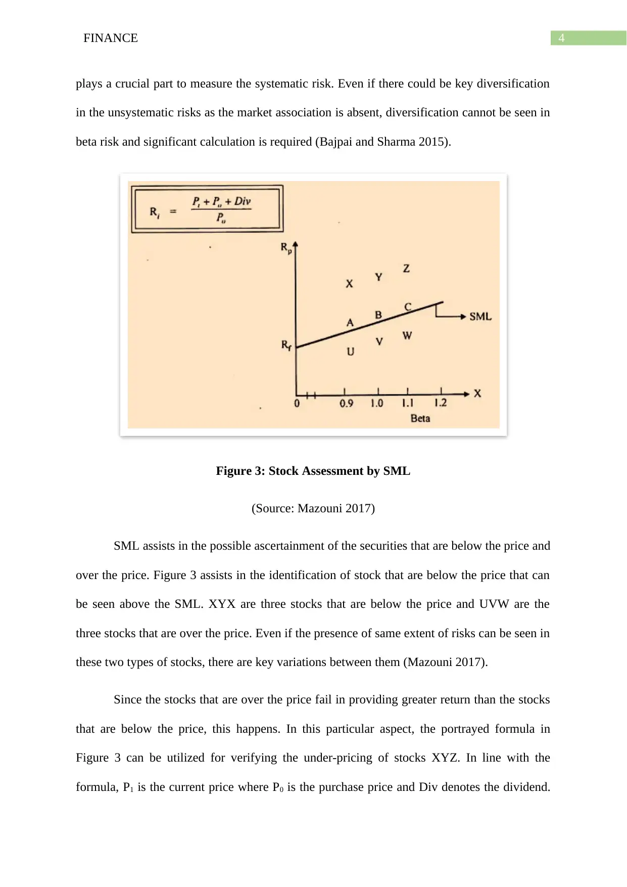
Figure 3: Stock Assessment by SML
(Source: Mazouni 2017)
SML assists in the possible ascertainment of the securities that are below the price and
over the price. Figure 3 assists in the identification of stock that are below the price that can
be seen above the SML. XYX are three stocks that are below the price and UVW are the
three stocks that are over the price. Even if the presence of same extent of risks can be seen in
these two types of stocks, there are key variations between them (Mazouni 2017).
Since the stocks that are over the price fail in providing greater return than the stocks
that are below the price, this happens. In this particular aspect, the portrayed formula in
Figure 3 can be utilized for verifying the under-pricing of stocks XYZ. In line with the
formula, P1 is the current price where P0 is the purchase price and Div denotes the dividend.
plays a crucial part to measure the systematic risk. Even if there could be key diversification
in the unsystematic risks as the market association is absent, diversification cannot be seen in
beta risk and significant calculation is required (Bajpai and Sharma 2015).
Figure 3: Stock Assessment by SML
(Source: Mazouni 2017)
SML assists in the possible ascertainment of the securities that are below the price and
over the price. Figure 3 assists in the identification of stock that are below the price that can
be seen above the SML. XYX are three stocks that are below the price and UVW are the
three stocks that are over the price. Even if the presence of same extent of risks can be seen in
these two types of stocks, there are key variations between them (Mazouni 2017).
Since the stocks that are over the price fail in providing greater return than the stocks
that are below the price, this happens. In this particular aspect, the portrayed formula in
Figure 3 can be utilized for verifying the under-pricing of stocks XYZ. In line with the
formula, P1 is the current price where P0 is the purchase price and Div denotes the dividend.

5FINANCE
The presence of ABC stocks can be seen in the SML which proves the accurateness of the
stock prices and same level of risk and return is carried by these stocks (Zhou, Simnett and
Green 2017).
Figure 4: Imperfect Market SML
(Source: Hong and Sraer 2016)
Stocks would be differently impacted in the non-availability of perfect information.
This happens because of the availability of all information in the perfect market where the
presence of the stocks can be seen on the SML. On the other hand, in the imperfect market,
the presence of a band can be seen in the SML rather than a single line. This can be depicted
from Figure 4 (Shaikh 2013).
The above discussion shows that SML is different from CML in different ways and
the summary of them are as follows.
1. In case of SML, the plotting of market risk as well as market return is done at an exact
timeframe; and a single line represents the whole line. CML is represented by a line
that involves in plotting return from a specific portfolio.
2. Risks and returns associated with the individual stocks are ascertained by the SML
while developing portfolio; but CML involves in the ascertainment of the risks and
returns associated with the efficient portfolios.
⊘ This is a preview!⊘
Do you want full access?
Subscribe today to unlock all pages.
Trusted by 1+ million students worldwide

6FINANCE
3. When considered efficiency, both the efficient as well as inefficient portfolios are
taken into account by SML; by only efficient portfolios are take into account by
CML.
4. In case of the measurement of risk, SML uses standard deviation where SML uses
beta (Han, Li and Li 2019).
Importance of Minimum Variance Portfolio
A minimum variance portfolio refers to such stock portfolio that the investors merge
in order to reduce the unpredictability in price of the overall portfolio. Unpredictability in
investments leads to the increase in market risk. These unpredictable increases and decreases
in stock price need to be reduced for the reduction in risks. The lower bond having
association with the efficient frontier is possible to be determined through the assistance of
minimum variance portfolio. There are certain portfolios that need to be inefficient even in
the presence of the fact that investments opportunities are carried by the portfolios. It means
equal risks are there in certain portfolios but variations can be seen in the returns of the
stocks. For this reason, portfolios staying under the minimum variance portfolio would not be
able to attract investors to invest in. Optimisation of systematic portfolio, improvement can
be brought in efficiency and diversification (Bodnar and Okhrin 2013). The following
discussion shows certain reasons that put major significance in the minimum variance
portfolio.
1. Factors such as social, environmental and governance are taken into consideration by
the investors when they make decisions regarding investments. This puts the
obligation on the firms to consider these criteria in order to sustain in the investment
sector. Some of the factors that require compliance by the auditors are green gas
emission, sustainability reporting and others. All these aspects are effectively
considered by minimum variance portfolio while developing the portfolio in order to
Paraphrase This Document
Need a fresh take? Get an instant paraphrase of this document with our AI Paraphraser

7FINANCE
provide necessary support to the investors to make investment decisions (Bodnar,
Mazur and Okhrin 2017).
2. It is possible to develop the risk parameters because of the fact that minimum risk
portfolio is the sole portfolio having reliance on the risk parameters. Therefore, the
investors become able in projecting over time with the help of econometric
techniques. This eliminates the necessity for projecting return (Xing, Hu and Yang
2014).
3. Average return is attained by the securities that have lower fluctuation of price. At the
same time, these attained returns are greater than the predicted return. In this process,
minimum variance portfolio plays a crucial part in appropriately implement low
volatility premium since this takes into consideration the relation between individual
investments.
4. It is possible for the investors to compare the risk-return ratio with the assistance of
the index in better manner as the efficient frontier lies near to the minimum variance
portfolio. Therefore, portfolio volatility is possible to be reduced along with the losses
in the presence of enhanced diversification (Bodnar, Parolya and Schmid 2018).
Reason for more Relevance of CAPM Equation than other Equations
The linear association between the required rate of return on investment and
systematic risk is called as Capital Asset Pricing Model (CAPM). It is denoted by a specific
formula that is shown below:

8FINANCE
Figure 6: Equation of CAPM
(Source: Dempsey 2013)
This particular formula in Figure 6 is largely utilized by the investors for the
ascertainment of the projected return on investments. This also provides major support to
assess the weighted average cost of capital that is used by the investors as a discount rate to
appraise investment proposals. The presence of certain assumptions can be seen in this that
needs to be taken into consideration and they are as follows:
1. The investment project must not be greater the firms which is investing.
2. The business operations of the proposed project and the investing firm need to be the
same.
3. The financing mix of the investing company’s capital structure and the proposed
project needs to be the same.
4. The same rates of return need to be maintained by the present providers of funds in
the investing company after undertaking the proposed project (Dempsey 2013).
In case there is not any change in the financial risk and business risk of the company after
undertaking the proposed investment project, the investors can use the discount rate on the
basis of the above-mentioned assumptions. Investors largely uses CAPM in order to get the
discount rate of a particular proposed investment project in case there are differences between
⊘ This is a preview!⊘
Do you want full access?
Subscribe today to unlock all pages.
Trusted by 1+ million students worldwide

9FINANCE
the risks associated with the project and the business risks associated with the firm. This
signifies the importance of CAPM in better investment decisions rather than the use of
weighted average cost of capital (Zabarankin, Pavlikov and Uryasev 2014). This is depicted
in the following figure:
Figure 7: CAPM or Weighted Average Cost of Capital
(Source: Kisman and Restiyanita 2015)
In line with Figure 7, an investor would not accept Project A in the presence of the
utilisation of weighted average cost of capital as the rate of discount because weighted
average cost of capital is higher than internal rate of return (IRR). However, it should not be
solely believe that this decision is correct at the time to make investment decisions. The
reason is the potting of the IRR of Project A over the head of SML and this can be seen at the
time of the use of discount rate of CAPM. It indicates towards the generation of greater return
by Project A as compared to the project that is needed to compensate the extent of systematic
risk. There would be enhancement in the shareholders’ value in case this is acknowledged
(Kisman and Restiyanita 2015).
Paraphrase This Document
Need a fresh take? Get an instant paraphrase of this document with our AI Paraphraser

10FINANCE
On the other hand, Project B needs to be suggested in line with weighted average cost
of capital which cannot be considered as a correct decision due to the rejection of the project
by CAPM rate of discount as there is not sufficient reward of the systematic risk by IRR (Oke
2013).
Some of the alternatives of CAPM are the growth model of Gordon, Fama French
model and dividend discount model as these models are used by the investors for enhancing
the process to make decisions. Critical assessments in the presence of statistical data are parts
of these models that make it difficult for the investors to make investment decisions.
Investors can get certain benefits by using the CAPM model. Systematic risk that is a reality
is considered by CAPM where different investors hold diversified portfolios and systematic
risk can be eliminated by this. CAPM provides the scope of computing cost of equity in a
better manner when compared with the dividend growth model because of the consideration
of systematic risk in the stock market. CAPM makes it possible to appraise the investment
projects in better manner by using calculation of the rate of discount (Oke 2013).
Conclusion
It can be seen from the above discussion that the investors are required to take into
consideration the aspects like SML, CML and minimum variance portfolio in order to make
the correct investment decisions. It can also be observed from the above discussion that it is
not feasible to make investment in the portfolios that stay under the minimum variance
portfolios. Investors can improve the efficiency and diversification of investment portfolios
with the assistance of systematic portfolio optimisation. Moreover, the above discussion also
shows the importance of CAPM to calculate the rate of return easily as compared to other
models. This helps in increasing the shareholder’s value.

11FINANCE
References
Bajpai, S. and Sharma, A.K., 2015. Capital asset pricing model and industry effect: Evidence
from Indian market. IUP Journal of Financial Risk Management, 12(2), p.30.
Bodnar, T. and Okhrin, Y., 2013. Boundaries of the risk aversion coefficient: Should we
invest in the global minimum variance portfolio?. Applied Mathematics and
Computation, 219(10), pp.5440-5448.
Bodnar, T., Mazur, S. and Okhrin, Y., 2017. Bayesian estimation of the global minimum
variance portfolio. European Journal of Operational Research, 256(1), pp.292-307.
Bodnar, T., Parolya, N. and Schmid, W., 2018. Estimation of the global minimum variance
portfolio in high dimensions. European Journal of Operational Research, 266(1), pp.371-
390.
Calvo, C., Ivorra, C. and Liern, V., 2016. Fuzzy portfolio selection with non-financial goals:
exploring the efficient frontier. Annals of Operations Research, 245(1-2), pp.31-46.
Dempsey, M., 2013. The capital asset pricing model (CAPM): the history of a failed
revolutionary idea in finance?. Abacus, 49, pp.7-23.
Han, X., Li, K. and Li, Y., 2019. Investor Overconfidence and the Security Market Line: New
Evidence from China. Macquarie University Faculty of Business & Economics Research
Paper.
Hong, H. and Sraer, D.A., 2016. Speculative betas. The Journal of Finance, 71(5), pp.2095-
2144.
Kisman, Z. and Restiyanita, S., 2015. M. The Validity of Capital Asset Pricing Model
(CAPM) and Arbitrage Pricing Theory (APT) in Predicting the Return of Stocks in Indonesia
⊘ This is a preview!⊘
Do you want full access?
Subscribe today to unlock all pages.
Trusted by 1+ million students worldwide
1 out of 13
Related Documents


Your All-in-One AI-Powered Toolkit for Academic Success.
+13062052269
info@desklib.com
Available 24*7 on WhatsApp / Email
![[object Object]](/_next/static/media/star-bottom.7253800d.svg)
Unlock your academic potential
Copyright © 2020–2026 A2Z Services. All Rights Reserved. Developed and managed by ZUCOL.