Semester 1, 2020: FIT3152 Assignment 2 - Australian Rainfall Analysis
VerifiedAdded on 2021/09/27
|29
|3405
|427
Project
AI Summary
This assignment focuses on analyzing Australian rainfall data to predict whether it will rain tomorrow. The project utilizes the "WAUS.csv" dataset, employing various classification models such as Decision Tree, Naïve Bayes, Bagging, Boosting, and Random Forest. The analysis includes data preprocessing to handle missing values and categorical attributes, followed by the creation of train and test datasets. The performance of each model is evaluated using confusion matrices, accuracy scores, ROC curves, and AUC values. The assignment identifies the most important variables for each model and concludes that Boosting is the best classifier based on both accuracy and AUC. The analysis is performed using R programming, and the results are presented with detailed explanations and visualizations. The analysis covers aspects like data exploration, preprocessing, model building, evaluation, and comparison, providing a comprehensive understanding of the data and the effectiveness of different classification techniques for rainfall prediction. The project also involves cross-validation and examination of the models' key variables.

FIT 3152: DATA ANALYTICS
Assignment 2 – Australian Rainfall Data
Name: Giridhar Gopal Sharma
Student ID: 29223709
Email: gsha0009@student.monash.edu
Semester 1 2020
Assignment 2 – Australian Rainfall Data
Name: Giridhar Gopal Sharma
Student ID: 29223709
Email: gsha0009@student.monash.edu
Semester 1 2020
Paraphrase This Document
Need a fresh take? Get an instant paraphrase of this document with our AI Paraphraser
Table of Contents
S No. Title
1. Overview
2. Task 1 and 2: Exploring Data/ Pre-Processing of Data
3. Task 3: Diving data into Train and Test sets
4. Task 4: Classification Models
5. Task 5: Confusion Matrix for each Model
6. Task 6: ROC curve and Area under curve (AUC)
7. Task 7: Combining and Commenting on results in Tasks 5 and 6
8. Task 8: Examining each of the Model
9. Task 9: Best Tree Classifier using Cross - Validation
10. Task 10: Artificial Neural Network (ANNs) Classifier
11. R-Codes
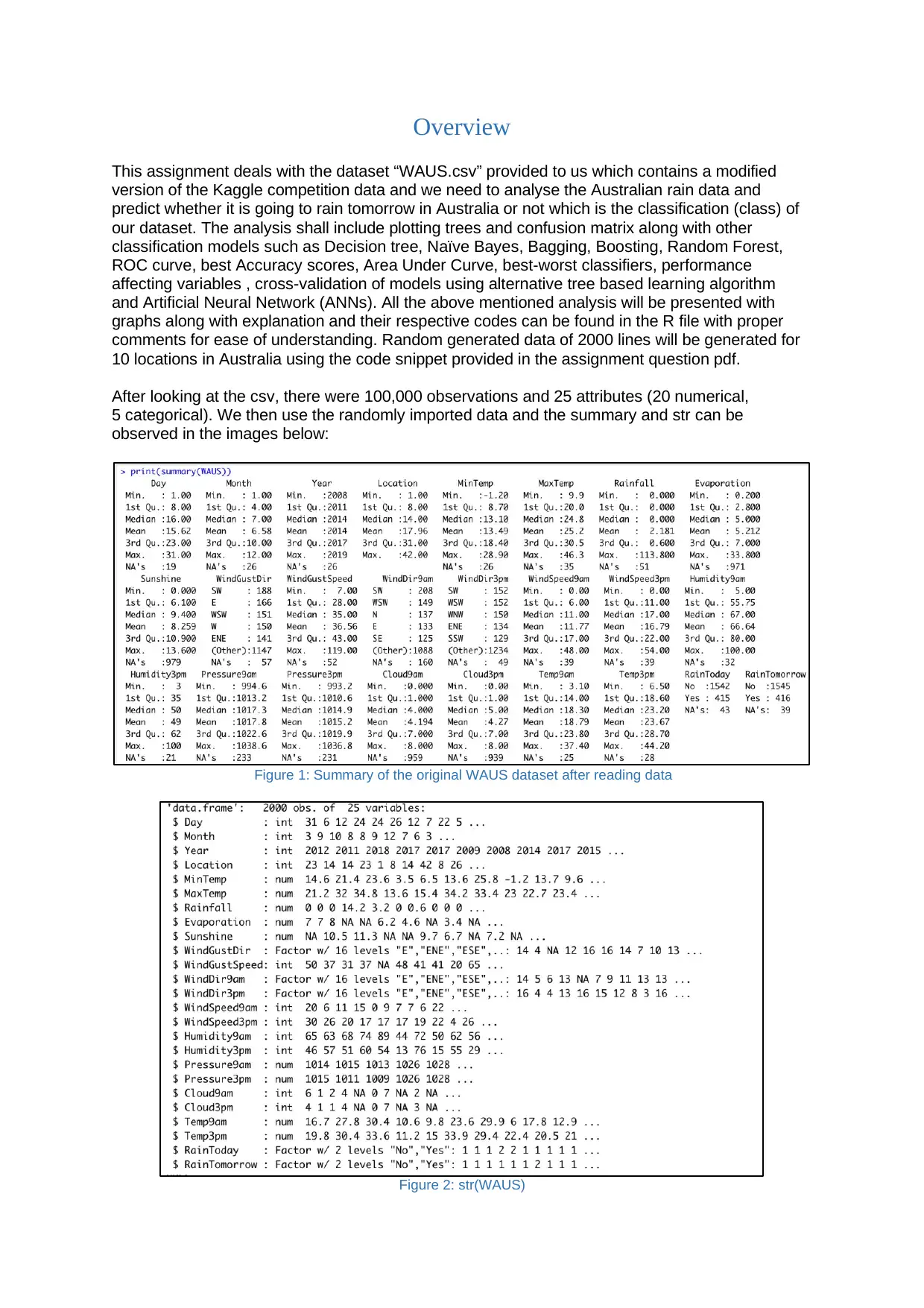
Overview
This assignment deals with the dataset “WAUS.csv” provided to us which contains a modified
version of the Kaggle competition data and we need to analyse the Australian rain data and
predict whether it is going to rain tomorrow in Australia or not which is the classification (class) of
our dataset. The analysis shall include plotting trees and confusion matrix along with other
classification models such as Decision tree, Naïve Bayes, Bagging, Boosting, Random Forest,
ROC curve, best Accuracy scores, Area Under Curve, best-worst classifiers, performance
affecting variables , cross-validation of models using alternative tree based learning algorithm
and Artificial Neural Network (ANNs). All the above mentioned analysis will be presented with
graphs along with explanation and their respective codes can be found in the R file with proper
comments for ease of understanding. Random generated data of 2000 lines will be generated for
10 locations in Australia using the code snippet provided in the assignment question pdf.
After looking at the csv, there were 100,000 observations and 25 attributes (20 numerical,
5 categorical). We then use the randomly imported data and the summary and str can be
observed in the images below:
Figure 1: Summary of the original WAUS dataset after reading data
Figure 2: str(WAUS)
⊘ This is a preview!⊘
Do you want full access?
Subscribe today to unlock all pages.
Trusted by 1+ million students worldwide
Task 1 and 2: Exploring Data/ Pre-Processing of Data
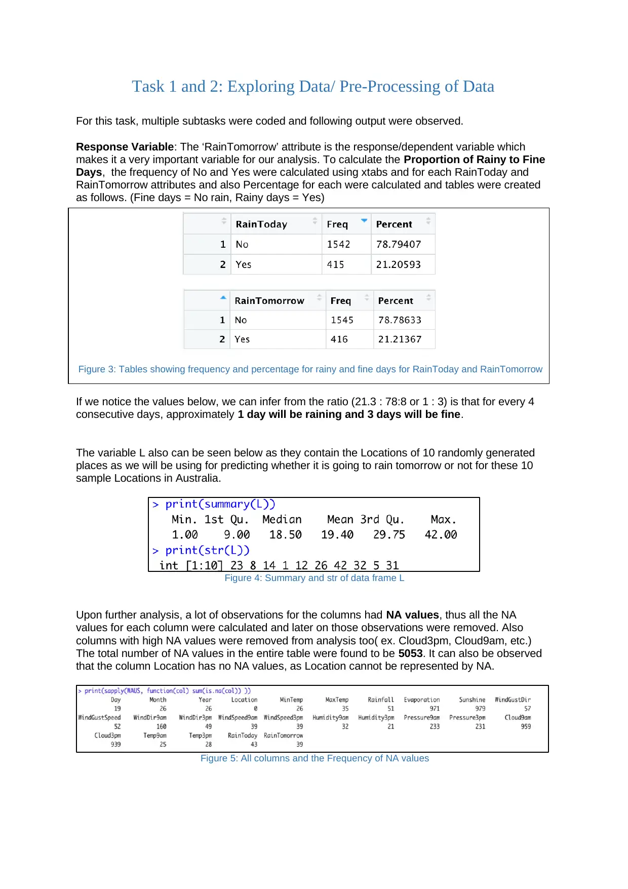
For this task, multiple subtasks were coded and following output were observed.
Response Variable: The ‘RainTomorrow’ attribute is the response/dependent variable which
makes it a very important variable for our analysis. To calculate the Proportion of Rainy to Fine
Days, the frequency of No and Yes were calculated using xtabs and for each RainToday and
RainTomorrow attributes and also Percentage for each were calculated and tables were created
as follows. (Fine days = No rain, Rainy days = Yes)
If we notice the values below, we can infer from the ratio (21.3 : 78:8 or 1 : 3) is that for every 4
consecutive days, approximately 1 day will be raining and 3 days will be fine.
The variable L also can be seen below as they contain the Locations of 10 randomly generated
places as we will be using for predicting whether it is going to rain tomorrow or not for these 10
sample Locations in Australia.
Figure 4: Summary and str of data frame L
Upon further analysis, a lot of observations for the columns had NA values, thus all the NA
values for each column were calculated and later on those observations were removed. Also
columns with high NA values were removed from analysis too( ex. Cloud3pm, Cloud9am, etc.)
The total number of NA values in the entire table were found to be 5053. It can also be observed
that the column Location has no NA values, as Location cannot be represented by NA.
Figure 5: All columns and the Frequency of NA values
Figure 3: Tables showing frequency and percentage for rainy and fine days for RainToday and RainTomorrow
Paraphrase This Document
Need a fresh take? Get an instant paraphrase of this document with our AI Paraphraser
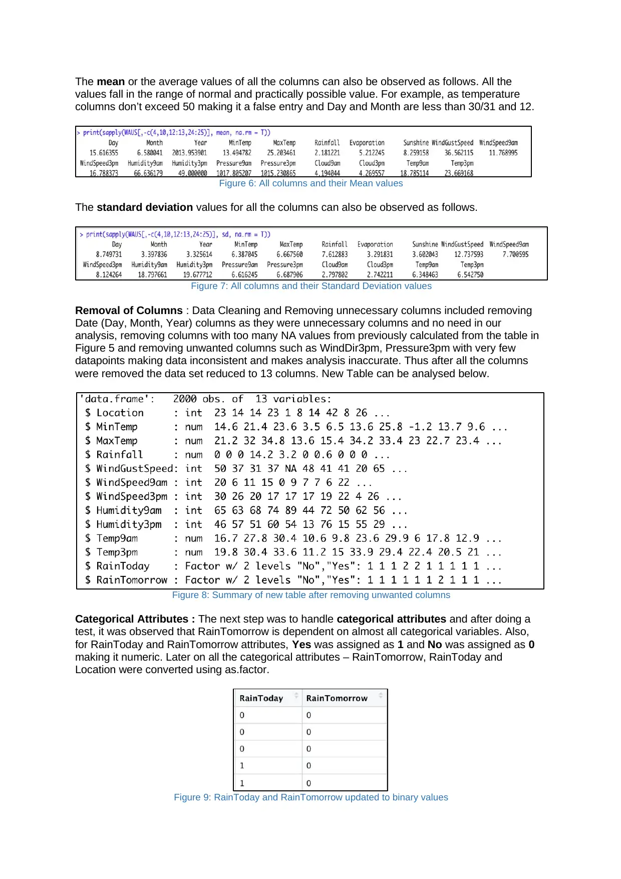
The mean or the average values of all the columns can also be observed as follows. All the
values fall in the range of normal and practically possible value. For example, as temperature
columns don’t exceed 50 making it a false entry and Day and Month are less than 30/31 and 12.
Figure 6: All columns and their Mean values
The standard deviation values for all the columns can also be observed as follows.
Figure 7: All columns and their Standard Deviation values
Removal of Columns : Data Cleaning and Removing unnecessary columns included removing
Date (Day, Month, Year) columns as they were unnecessary columns and no need in our
analysis, removing columns with too many NA values from previously calculated from the table in
Figure 5 and removing unwanted columns such as WindDir3pm, Pressure3pm with very few
datapoints making data inconsistent and makes analysis inaccurate. Thus after all the columns
were removed the data set reduced to 13 columns. New Table can be analysed below.
Figure 8: Summary of new table after removing unwanted columns
Categorical Attributes : The next step was to handle categorical attributes and after doing a
test, it was observed that RainTomorrow is dependent on almost all categorical variables. Also,
for RainToday and RainTomorrow attributes, Yes was assigned as 1 and No was assigned as 0
making it numeric. Later on all the categorical attributes – RainTomorrow, RainToday and
Location were converted using as.factor.
Figure 9: RainToday and RainTomorrow updated to binary values
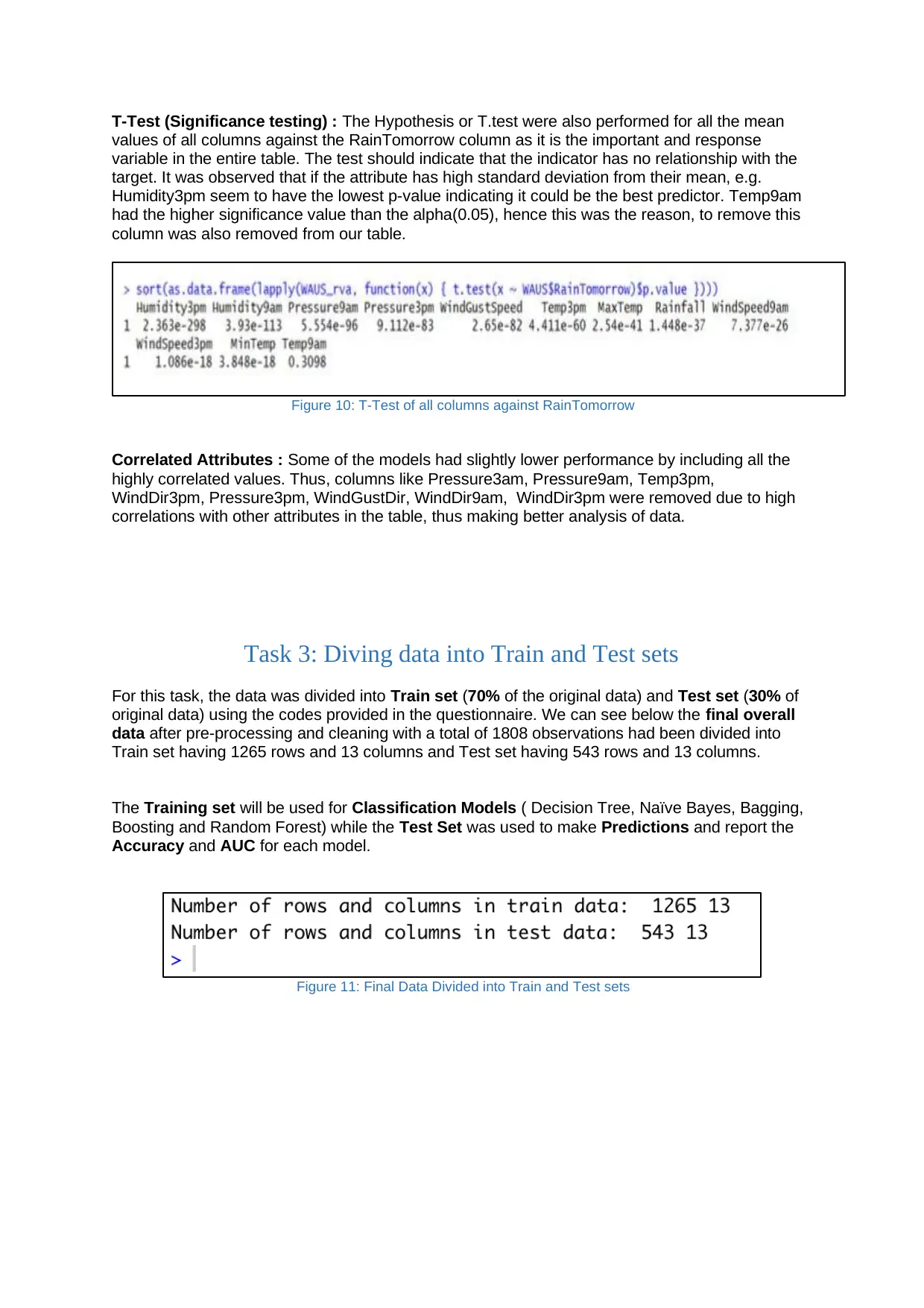
T-Test (Significance testing) : The Hypothesis or T.test were also performed for all the mean
values of all columns against the RainTomorrow column as it is the important and response
variable in the entire table. The test should indicate that the indicator has no relationship with the
target. It was observed that if the attribute has high standard deviation from their mean, e.g.
Humidity3pm seem to have the lowest p-value indicating it could be the best predictor. Temp9am
had the higher significance value than the alpha(0.05), hence this was the reason, to remove this
column was also removed from our table.
Figure 10: T-Test of all columns against RainTomorrow
Correlated Attributes : Some of the models had slightly lower performance by including all the
highly correlated values. Thus, columns like Pressure3am, Pressure9am, Temp3pm,
WindDir3pm, Pressure3pm, WindGustDir, WindDir9am, WindDir3pm were removed due to high
correlations with other attributes in the table, thus making better analysis of data.
Task 3: Diving data into Train and Test sets
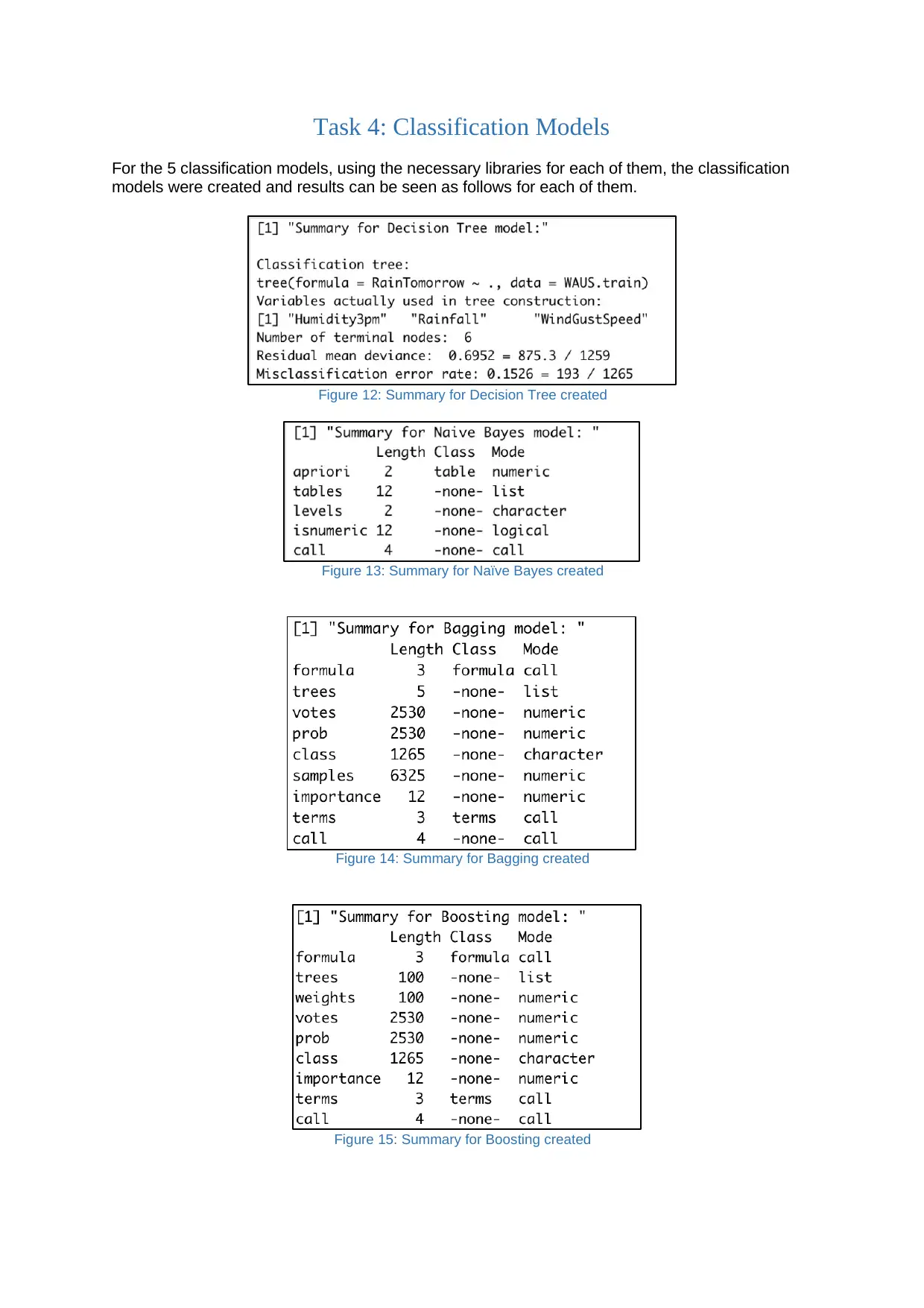
For this task, the data was divided into Train set (70% of the original data) and Test set (30% of
original data) using the codes provided in the questionnaire. We can see below the final overall
data after pre-processing and cleaning with a total of 1808 observations had been divided into
Train set having 1265 rows and 13 columns and Test set having 543 rows and 13 columns.
The Training set will be used for Classification Models ( Decision Tree, Naïve Bayes, Bagging,
Boosting and Random Forest) while the Test Set was used to make Predictions and report the
Accuracy and AUC for each model.
Figure 11: Final Data Divided into Train and Test sets
values of all columns against the RainTomorrow column as it is the important and response
variable in the entire table. The test should indicate that the indicator has no relationship with the
target. It was observed that if the attribute has high standard deviation from their mean, e.g.
Humidity3pm seem to have the lowest p-value indicating it could be the best predictor. Temp9am
had the higher significance value than the alpha(0.05), hence this was the reason, to remove this
column was also removed from our table.
Figure 10: T-Test of all columns against RainTomorrow
Correlated Attributes : Some of the models had slightly lower performance by including all the
highly correlated values. Thus, columns like Pressure3am, Pressure9am, Temp3pm,
WindDir3pm, Pressure3pm, WindGustDir, WindDir9am, WindDir3pm were removed due to high
correlations with other attributes in the table, thus making better analysis of data.
Task 3: Diving data into Train and Test sets
For this task, the data was divided into Train set (70% of the original data) and Test set (30% of
original data) using the codes provided in the questionnaire. We can see below the final overall
data after pre-processing and cleaning with a total of 1808 observations had been divided into
Train set having 1265 rows and 13 columns and Test set having 543 rows and 13 columns.
The Training set will be used for Classification Models ( Decision Tree, Naïve Bayes, Bagging,
Boosting and Random Forest) while the Test Set was used to make Predictions and report the
Accuracy and AUC for each model.
Figure 11: Final Data Divided into Train and Test sets
⊘ This is a preview!⊘
Do you want full access?
Subscribe today to unlock all pages.
Trusted by 1+ million students worldwide
Task 4: Classification Models
For the 5 classification models, using the necessary libraries for each of them, the classification
models were created and results can be seen as follows for each of them.
Figure 12: Summary for Decision Tree created
Figure 13: Summary for Naïve Bayes created
Figure 14: Summary for Bagging created
Figure 15: Summary for Boosting created
Paraphrase This Document
Need a fresh take? Get an instant paraphrase of this document with our AI Paraphraser
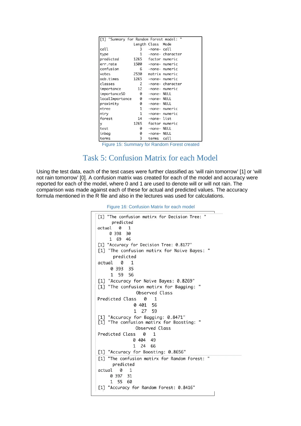
Figure 15: Summary for Random Forest created
Task 5: Confusion Matrix for each Model
Using the test data, each of the test cases were further classified as ‘will rain tomorrow’ [1] or ‘will
not rain tomorrow’ [0]. A confusion matrix was created for each of the model and accuracy were
reported for each of the model, where 0 and 1 are used to denote will or will not rain. The
comparison was made against each of these for actual and predicted values. The accuracy
formula mentioned in the R file and also in the lectures was used for calculations.
Figure 16: Confusion Matrix for each model
From confusion matrix and accuracy, the order of accuracy in decreasing order is:
Boosting > Bagging > Random Forest > Naïve Bayes > Decision Tree
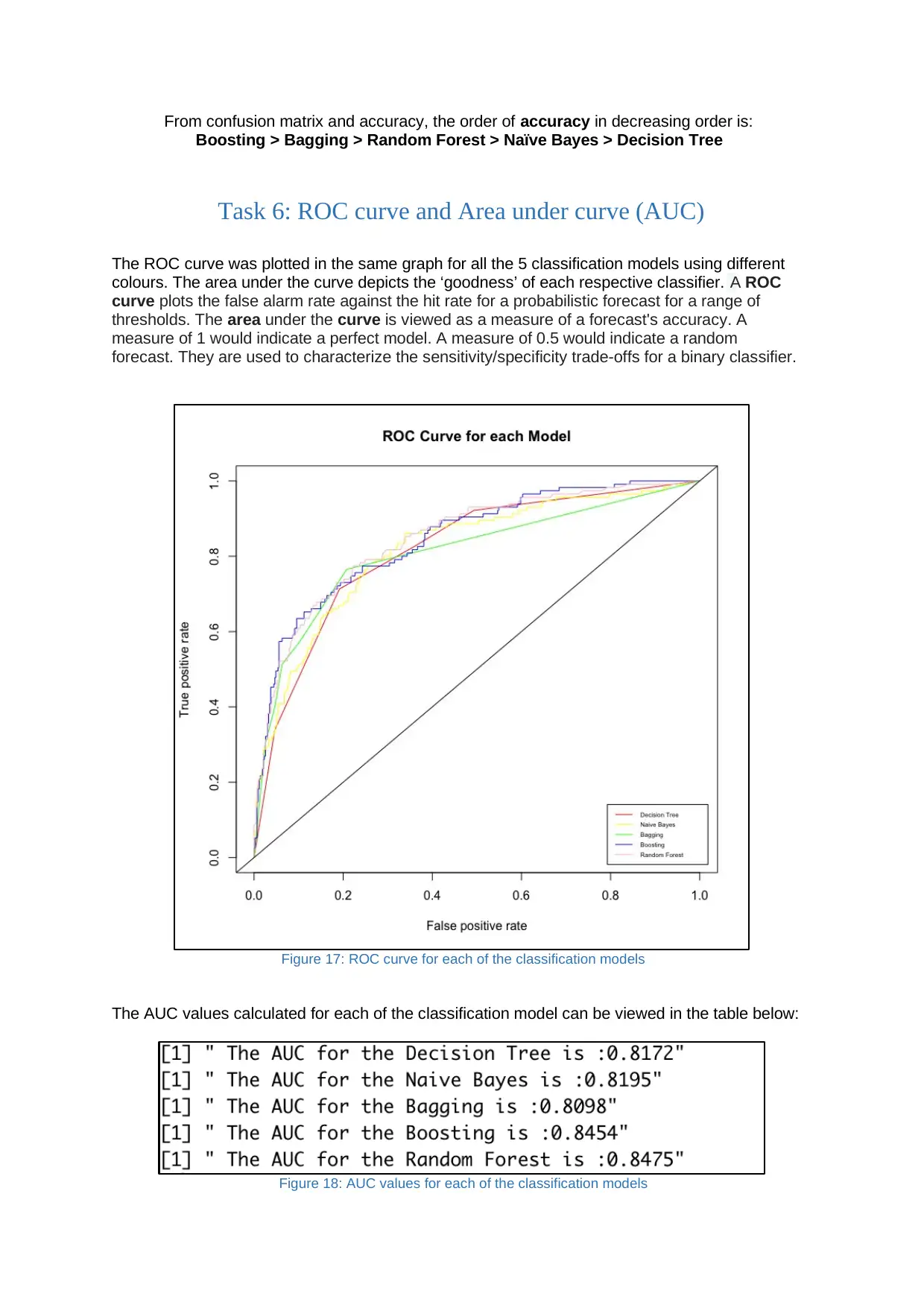
Task 6: ROC curve and Area under curve (AUC)
The ROC curve was plotted in the same graph for all the 5 classification models using different
colours. The area under the curve depicts the ‘goodness’ of each respective classifier. A ROC
curve plots the false alarm rate against the hit rate for a probabilistic forecast for a range of
thresholds. The area under the curve is viewed as a measure of a forecast's accuracy. A
measure of 1 would indicate a perfect model. A measure of 0.5 would indicate a random
forecast. They are used to characterize the sensitivity/specificity trade-offs for a binary classifier.
Figure 17: ROC curve for each of the classification models
The AUC values calculated for each of the classification model can be viewed in the table below:
Figure 18: AUC values for each of the classification models
Boosting > Bagging > Random Forest > Naïve Bayes > Decision Tree
Task 6: ROC curve and Area under curve (AUC)
The ROC curve was plotted in the same graph for all the 5 classification models using different
colours. The area under the curve depicts the ‘goodness’ of each respective classifier. A ROC
curve plots the false alarm rate against the hit rate for a probabilistic forecast for a range of
thresholds. The area under the curve is viewed as a measure of a forecast's accuracy. A
measure of 1 would indicate a perfect model. A measure of 0.5 would indicate a random
forecast. They are used to characterize the sensitivity/specificity trade-offs for a binary classifier.
Figure 17: ROC curve for each of the classification models
The AUC values calculated for each of the classification model can be viewed in the table below:
Figure 18: AUC values for each of the classification models
⊘ This is a preview!⊘
Do you want full access?
Subscribe today to unlock all pages.
Trusted by 1+ million students worldwide
Task 7: Combining and Commenting on results in Tasks 5 and 6
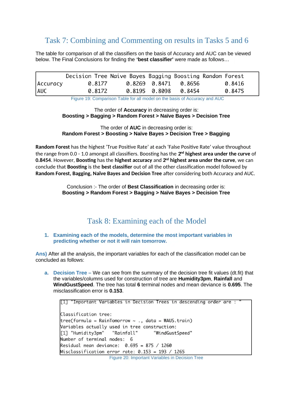
The table for comparison of all the classifiers on the basis of Accuracy and AUC can be viewed
below. The Final Conclusions for finding the ‘best classifier’ were made as follows…
Figure 19: Comparison Table for all model on the basis of Accuracy and AUC
The order of Accuracy in decreasing order is:
Boosting > Bagging > Random Forest > Naïve Bayes > Decision Tree
The order of AUC in decreasing order is:
Random Forest > Boosting > Naïve Bayes > Decision Tree > Bagging
Random Forest has the highest ‘True Positive Rate’ at each ‘False Positive Rate’ value throughout
the range from 0.0 - 1.0 amongst all classifiers. Boosting has the 2nd highest area under the curve of
0.8454. However, Boosting has the highest accuracy and 2nd highest area under the curve, we can
conclude that Boosting is the best classifier out of all the other classification model followed by
Random Forest, Bagging, Naïve Bayes and Decision Tree after considering both Accuracy and AUC.
Conclusion :- The order of Best Classification in decreasing order is:
Boosting > Random Forest > Bagging > Naïve Bayes > Decision Tree
Task 8: Examining each of the Model
1. Examining each of the models, determine the most important variables in
predicting whether or not it will rain tomorrow.
Ans) After all the analysis, the important variables for each of the classification model can be
concluded as follows:
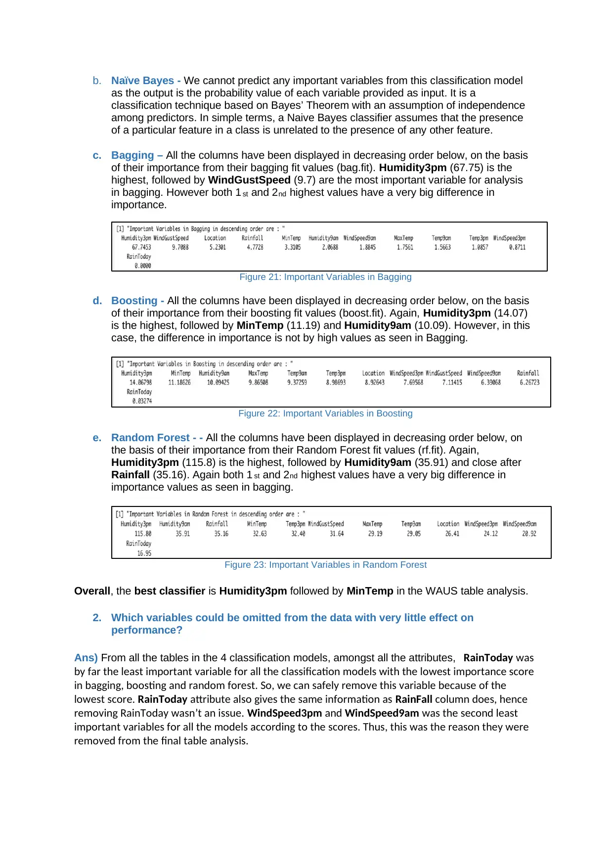
a. Decision Tree – We can see from the summary of the decision tree fit values (dt.fit) that
the variables/columns used for construction of tree are Humidity3pm, Rainfall and
WindGustSpeed. The tree has total 6 terminal nodes and mean deviance is 0.695. The
misclassification error is 0.153.
Figure 20: Important Variables in Decision Tree
The table for comparison of all the classifiers on the basis of Accuracy and AUC can be viewed
below. The Final Conclusions for finding the ‘best classifier’ were made as follows…
Figure 19: Comparison Table for all model on the basis of Accuracy and AUC
The order of Accuracy in decreasing order is:
Boosting > Bagging > Random Forest > Naïve Bayes > Decision Tree
The order of AUC in decreasing order is:
Random Forest > Boosting > Naïve Bayes > Decision Tree > Bagging
Random Forest has the highest ‘True Positive Rate’ at each ‘False Positive Rate’ value throughout
the range from 0.0 - 1.0 amongst all classifiers. Boosting has the 2nd highest area under the curve of
0.8454. However, Boosting has the highest accuracy and 2nd highest area under the curve, we can
conclude that Boosting is the best classifier out of all the other classification model followed by
Random Forest, Bagging, Naïve Bayes and Decision Tree after considering both Accuracy and AUC.
Conclusion :- The order of Best Classification in decreasing order is:
Boosting > Random Forest > Bagging > Naïve Bayes > Decision Tree
Task 8: Examining each of the Model
1. Examining each of the models, determine the most important variables in
predicting whether or not it will rain tomorrow.
Ans) After all the analysis, the important variables for each of the classification model can be
concluded as follows:
a. Decision Tree – We can see from the summary of the decision tree fit values (dt.fit) that
the variables/columns used for construction of tree are Humidity3pm, Rainfall and
WindGustSpeed. The tree has total 6 terminal nodes and mean deviance is 0.695. The
misclassification error is 0.153.
Figure 20: Important Variables in Decision Tree
Paraphrase This Document
Need a fresh take? Get an instant paraphrase of this document with our AI Paraphraser
b. Naïve Bayes - We cannot predict any important variables from this classification model
as the output is the probability value of each variable provided as input. It is a
classification technique based on Bayes’ Theorem with an assumption of independence
among predictors. In simple terms, a Naive Bayes classifier assumes that the presence
of a particular feature in a class is unrelated to the presence of any other feature.
c. Bagging – All the columns have been displayed in decreasing order below, on the basis
of their importance from their bagging fit values (bag.fit). Humidity3pm (67.75) is the
highest, followed by WindGustSpeed (9.7) are the most important variable for analysis
in bagging. However both 1 st and 2nd highest values have a very big difference in
importance.
Figure 21: Important Variables in Bagging
d. Boosting - All the columns have been displayed in decreasing order below, on the basis
of their importance from their boosting fit values (boost.fit). Again, Humidity3pm (14.07)
is the highest, followed by MinTemp (11.19) and Humidity9am (10.09). However, in this
case, the difference in importance is not by high values as seen in Bagging.
Figure 22: Important Variables in Boosting
e. Random Forest - - All the columns have been displayed in decreasing order below, on
the basis of their importance from their Random Forest fit values (rf.fit). Again,
Humidity3pm (115.8) is the highest, followed by Humidity9am (35.91) and close after
Rainfall (35.16). Again both 1 st and 2nd highest values have a very big difference in
importance values as seen in bagging.
Figure 23: Important Variables in Random Forest
Overall, the best classifier is Humidity3pm followed by MinTemp in the WAUS table analysis.
2. Which variables could be omitted from the data with very little effect on
performance?
Ans) From all the tables in the 4 classification models, amongst all the attributes, RainToday was
by far the least important variable for all the classification models with the lowest importance score
in bagging, boosting and random forest. So, we can safely remove this variable because of the
lowest score. RainToday attribute also gives the same information as RainFall column does, hence
removing RainToday wasn’t an issue. WindSpeed3pm and WindSpeed9am was the second least
important variables for all the models according to the scores. Thus, this was the reason they were
removed from the final table analysis.
Task 9: Best Tree Classifier using Cross – Validation
Once all the classification models were created in Task4 , for Improving the Accuracy, various
experiments on existing classifiers were performed to make it the best classifier out of all the
ones with Highest Accuracy and Highest AUC values. For this, the best classifier among all
the 5 models, Random Forest was selected and task cross validation was done. The
conclusions were made, whether the Accuracy could be further improved or not.
Factors important for choosing this model: Highest Accuracy and Highest AUC values required.
Best Classifier : Random Forest
Results: For this, basically overfitting of data was done for Random Forest; the Fit data was
divided into k subsets and then each of the k subsets were trained on k-1 partitions, whereas
the last part was used for testing. This was done using the K-fold cv function. Building (or
training) the Random Forest model was done using the remaining part of the data set Test as
mentioned above after diving the Fit data. Further, the effectiveness of the model on the
reserved sample of the data set is compared. In our case, the training/ testing data as divided in
the beginning and later used to create fit data for Random Forest were used.
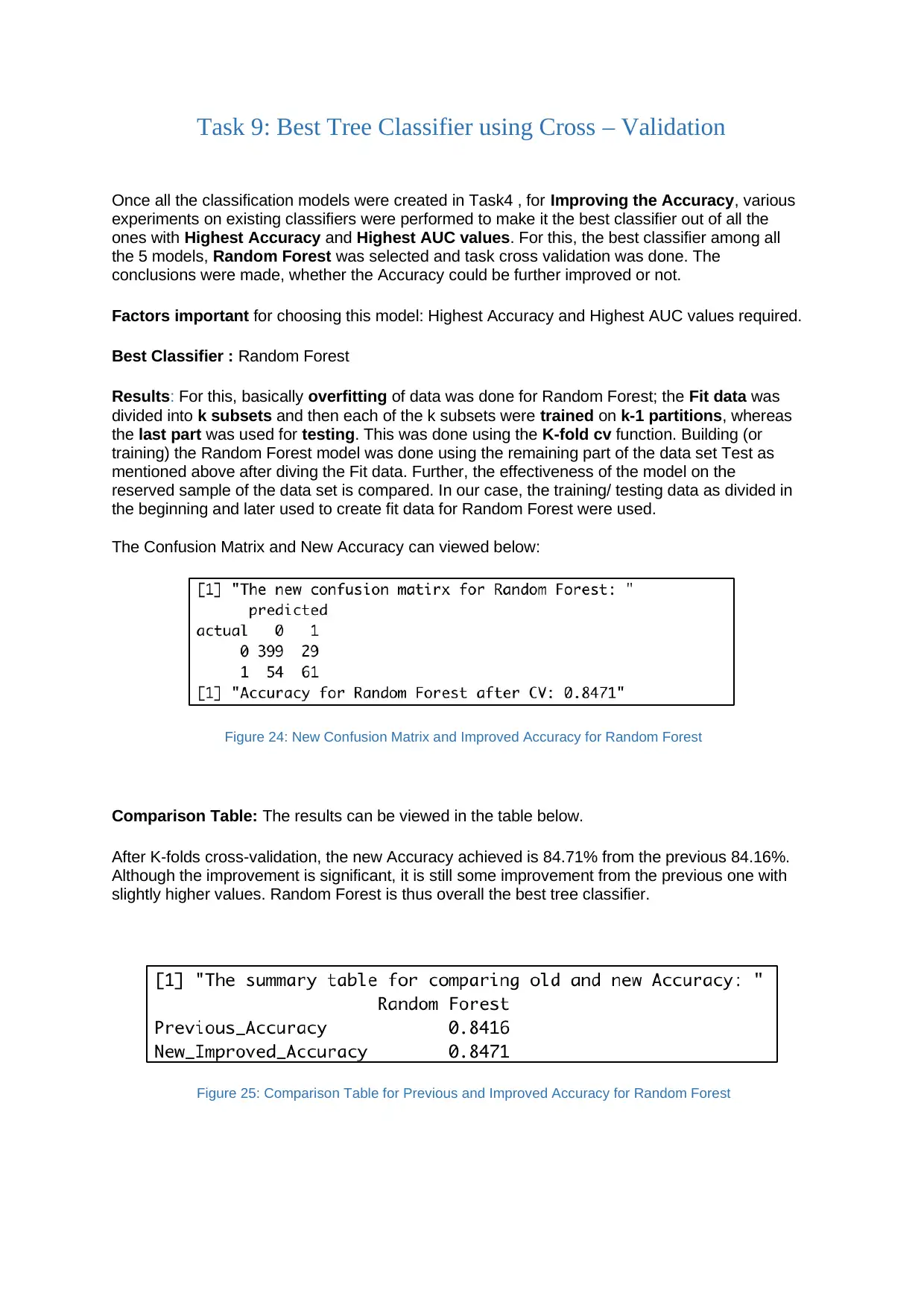
The Confusion Matrix and New Accuracy can viewed below:
Figure 24: New Confusion Matrix and Improved Accuracy for Random Forest
Comparison Table: The results can be viewed in the table below.
After K-folds cross-validation, the new Accuracy achieved is 84.71% from the previous 84.16%.
Although the improvement is significant, it is still some improvement from the previous one with
slightly higher values. Random Forest is thus overall the best tree classifier.
Figure 25: Comparison Table for Previous and Improved Accuracy for Random Forest
Once all the classification models were created in Task4 , for Improving the Accuracy, various
experiments on existing classifiers were performed to make it the best classifier out of all the
ones with Highest Accuracy and Highest AUC values. For this, the best classifier among all
the 5 models, Random Forest was selected and task cross validation was done. The
conclusions were made, whether the Accuracy could be further improved or not.
Factors important for choosing this model: Highest Accuracy and Highest AUC values required.
Best Classifier : Random Forest
Results: For this, basically overfitting of data was done for Random Forest; the Fit data was
divided into k subsets and then each of the k subsets were trained on k-1 partitions, whereas
the last part was used for testing. This was done using the K-fold cv function. Building (or
training) the Random Forest model was done using the remaining part of the data set Test as
mentioned above after diving the Fit data. Further, the effectiveness of the model on the
reserved sample of the data set is compared. In our case, the training/ testing data as divided in
the beginning and later used to create fit data for Random Forest were used.
The Confusion Matrix and New Accuracy can viewed below:
Figure 24: New Confusion Matrix and Improved Accuracy for Random Forest
Comparison Table: The results can be viewed in the table below.
After K-folds cross-validation, the new Accuracy achieved is 84.71% from the previous 84.16%.
Although the improvement is significant, it is still some improvement from the previous one with
slightly higher values. Random Forest is thus overall the best tree classifier.
Figure 25: Comparison Table for Previous and Improved Accuracy for Random Forest
⊘ This is a preview!⊘
Do you want full access?
Subscribe today to unlock all pages.
Trusted by 1+ million students worldwide
1 out of 29

Your All-in-One AI-Powered Toolkit for Academic Success.
+13062052269
info@desklib.com
Available 24*7 on WhatsApp / Email
![[object Object]](/_next/static/media/star-bottom.7253800d.svg)
Unlock your academic potential
Copyright © 2020–2026 A2Z Services. All Rights Reserved. Developed and managed by ZUCOL.