Foundation Skills in Data Analysis

This document provides an introduction to statistical analysis and explores the relationship between variables in data analysis. It discusses correlation and regression analysis, as well as time series analysis. The document also includes examples and explanations of how to estimate house prices using regression models.

FOUNDATION SKILLS IN DATA ANALYSIS
STUDENT ID:
[Pick the date]

Introduction
Statistical analysis is a useful tool which can either be used to summarise and find
relationship between the given variables or estimate population parameter. For the given task,
the focus is on descriptive statistics and hence prediction about population parameters is not
required. The objective of the given report is to use the correlation and regression analysis for
carrying out the sample data analysis to estimate the values of the dependent variables and
estimation of the underlying nature of relationship between selected variables. Also, time
series analysis has been carried out for median prices in Melbourne based on the sample data
provided.
Relationships
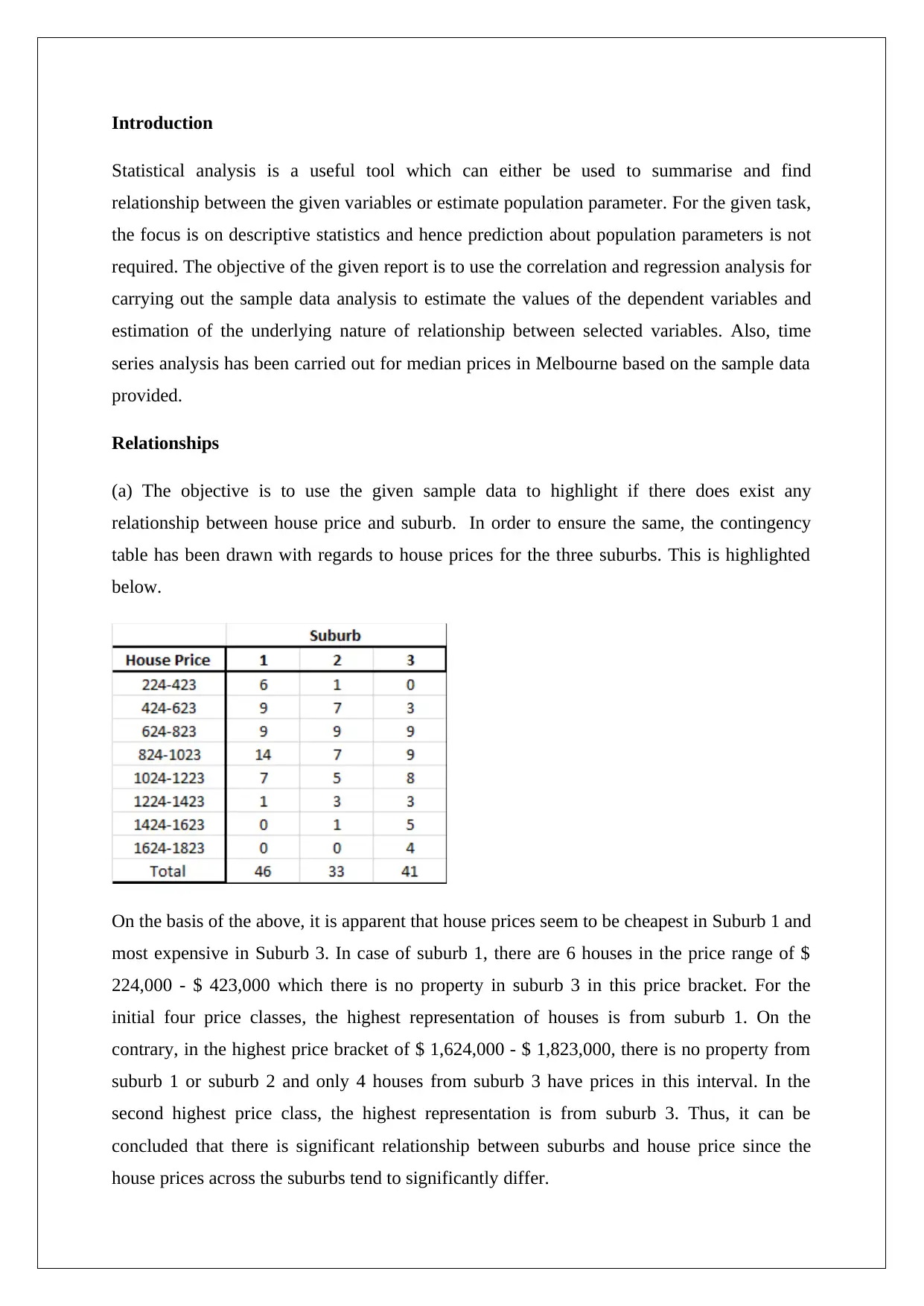
(a) The objective is to use the given sample data to highlight if there does exist any
relationship between house price and suburb. In order to ensure the same, the contingency
table has been drawn with regards to house prices for the three suburbs. This is highlighted
below.
On the basis of the above, it is apparent that house prices seem to be cheapest in Suburb 1 and
most expensive in Suburb 3. In case of suburb 1, there are 6 houses in the price range of $
224,000 - $ 423,000 which there is no property in suburb 3 in this price bracket. For the
initial four price classes, the highest representation of houses is from suburb 1. On the
contrary, in the highest price bracket of $ 1,624,000 - $ 1,823,000, there is no property from
suburb 1 or suburb 2 and only 4 houses from suburb 3 have prices in this interval. In the
second highest price class, the highest representation is from suburb 3. Thus, it can be
concluded that there is significant relationship between suburbs and house price since the
house prices across the suburbs tend to significantly differ.

(b) The objective is to highlight based on the sample data if the underlying relationship
between each of the independent variables ( i.e. LandSizeSqm, HouseAreaSqm,
WeeklyRent ) and the dependent variable i.e. HousePrice is linear or non-linear. The
appropriate tool to analyse the same would be scatter plot between the independent and
dependent variable chosen.
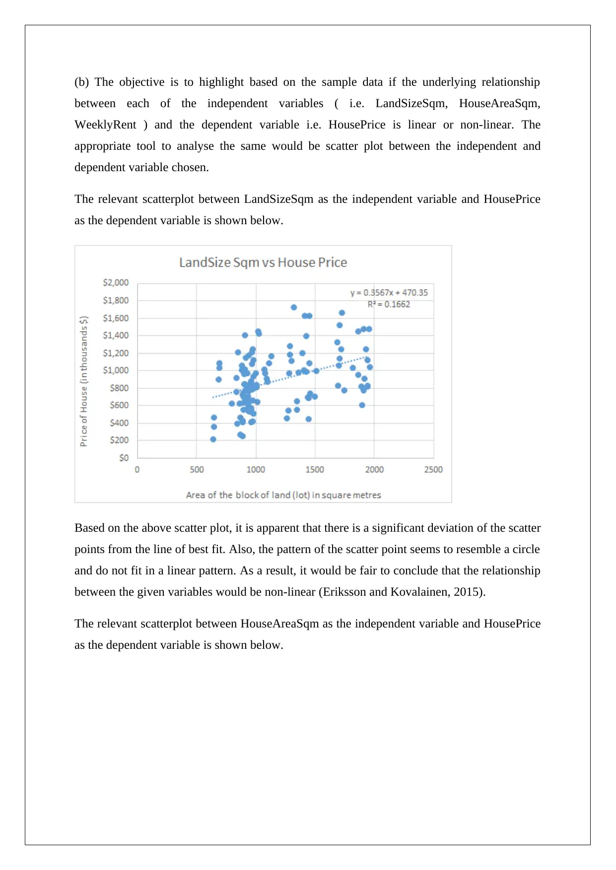
The relevant scatterplot between LandSizeSqm as the independent variable and HousePrice
as the dependent variable is shown below.
Based on the above scatter plot, it is apparent that there is a significant deviation of the scatter
points from the line of best fit. Also, the pattern of the scatter point seems to resemble a circle
and do not fit in a linear pattern. As a result, it would be fair to conclude that the relationship
between the given variables would be non-linear (Eriksson and Kovalainen, 2015).
The relevant scatterplot between HouseAreaSqm as the independent variable and HousePrice
as the dependent variable is shown below.

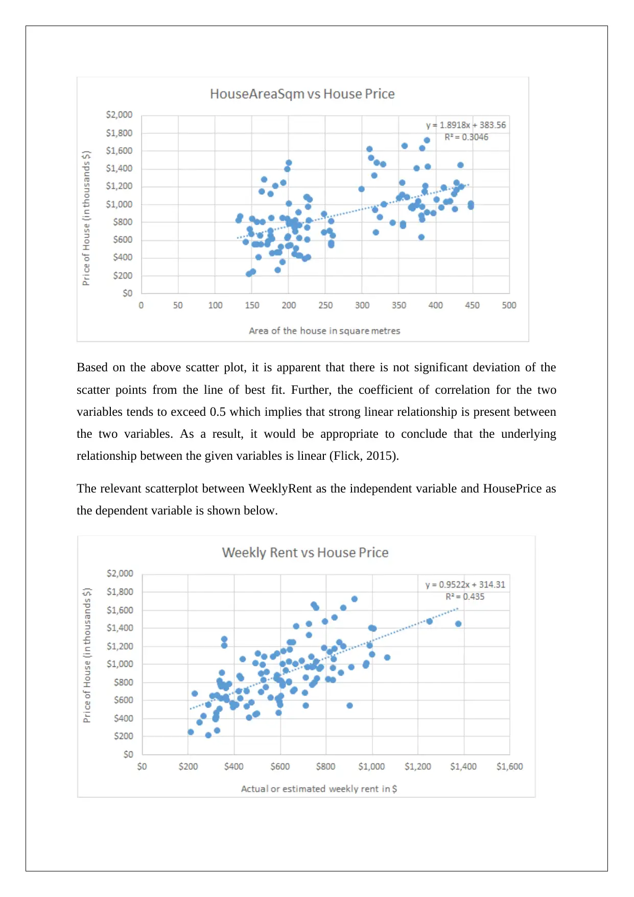
Based on the above scatter plot, it is apparent that there is not significant deviation of the
scatter points from the line of best fit. Further, the coefficient of correlation for the two
variables tends to exceed 0.5 which implies that strong linear relationship is present between
the two variables. As a result, it would be appropriate to conclude that the underlying
relationship between the given variables is linear (Flick, 2015).
The relevant scatterplot between WeeklyRent as the independent variable and HousePrice as
the dependent variable is shown below.

Based on the above scatter plot, it is apparent that there is not significant deviation of the
scatter points from the line of best fit. Further, the coefficient of correlation for the two
variables tends to exceed 0.6 which implies that strong linear relationship is present between
the two variables. As a result, it would be appropriate to conclude that the underlying
relationship between the given variables is linear (Hair et. al., 2015).
(c) The coefficient of determination or R2 can act as an indicator of the underlying strength of
relationship between the three independent variables and one dependent variable. Comparing
the R2 of the three scatter plots obtained above, it can be inferred that the independent
variable weekly rent has the strongest relationship with house price as the underlying
coefficient of determination is the highest amongst the three available models (Medhi, 2016).
Regression Analysis
(a) Regression analysis is a useful tool which is used to establish a linear relationship
between an independent variable and dependent variable based on which the estimation of
dependent variable for different values of independent variable can be done (Lieberman et.
al., 2013). In this case, the objective is to estimate a simple linear regression model with
HouseAreaSqm as the independent variable and HousePrice as the dependent variable. The
sample data provided would be used to achieve the same. The regression model output
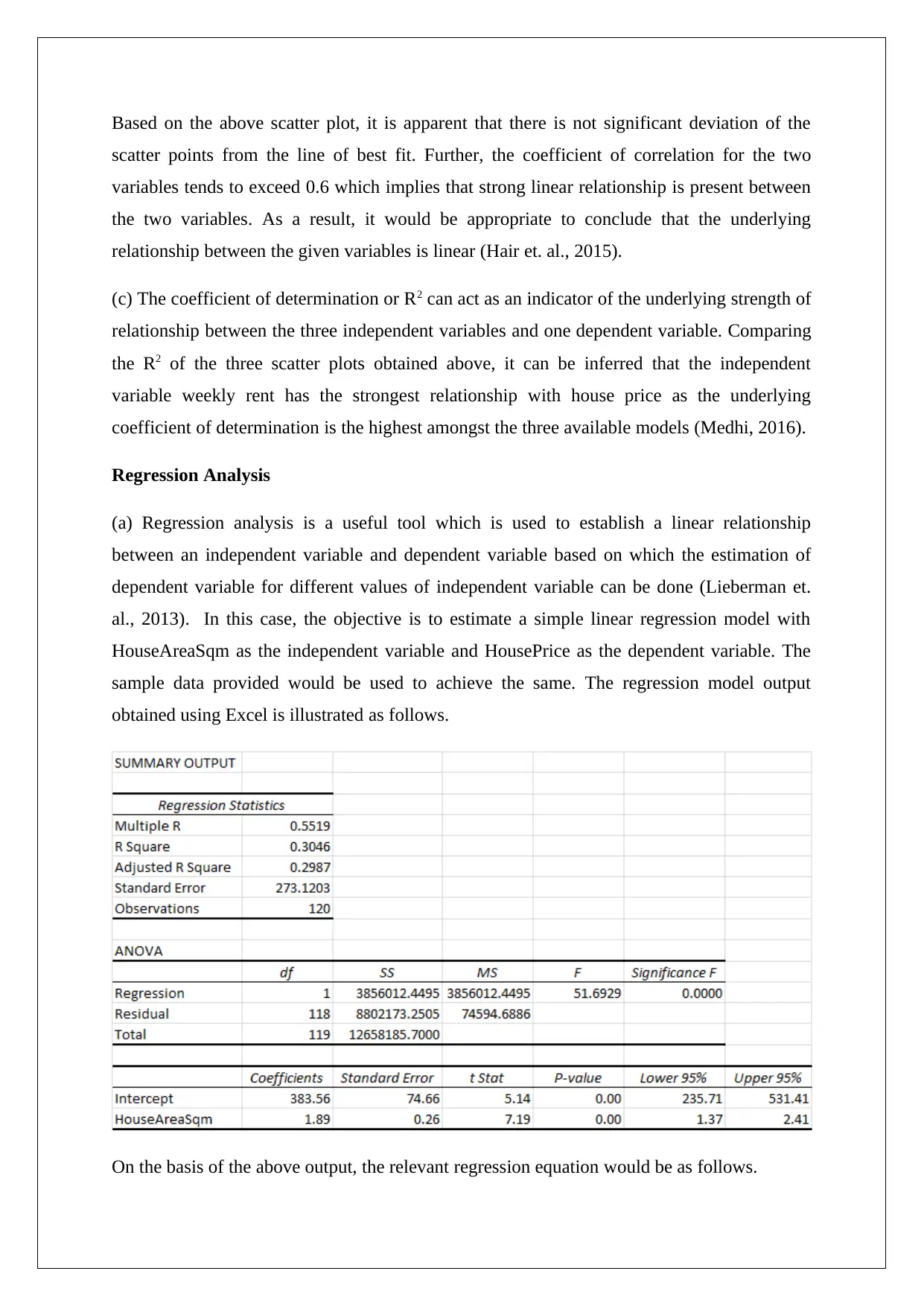
obtained using Excel is illustrated as follows.
On the basis of the above output, the relevant regression equation would be as follows.

House Price ($ 000’s) = 383.56 + 1.89*HouseAreaSqm
In the above model, the intercept is 383.56 while the slope value is 1.89.
The objective is to estimate the house price of a house with area of 500 square meters using
the above equation which can be done by substituting the value of HouseAreaSqm as 500.
House Price ($ 000’s) = 383.56 + 1.89*500 = 1329.46
The major concern with regards to the above estimate is that it may not be accurate since the
value of house area (i.e. 500 square meters) does not lie in the range of independent variable
values which has been used for the estimation of regression model. The extrapolation of
values for those independent variables value which lie outside the range of values used to
construct the regression model is not considered a healthy practice and often leads to
unreliable results which would be a key concern in this case also (Hastie, Tibshirani and
Friedman, 2016).
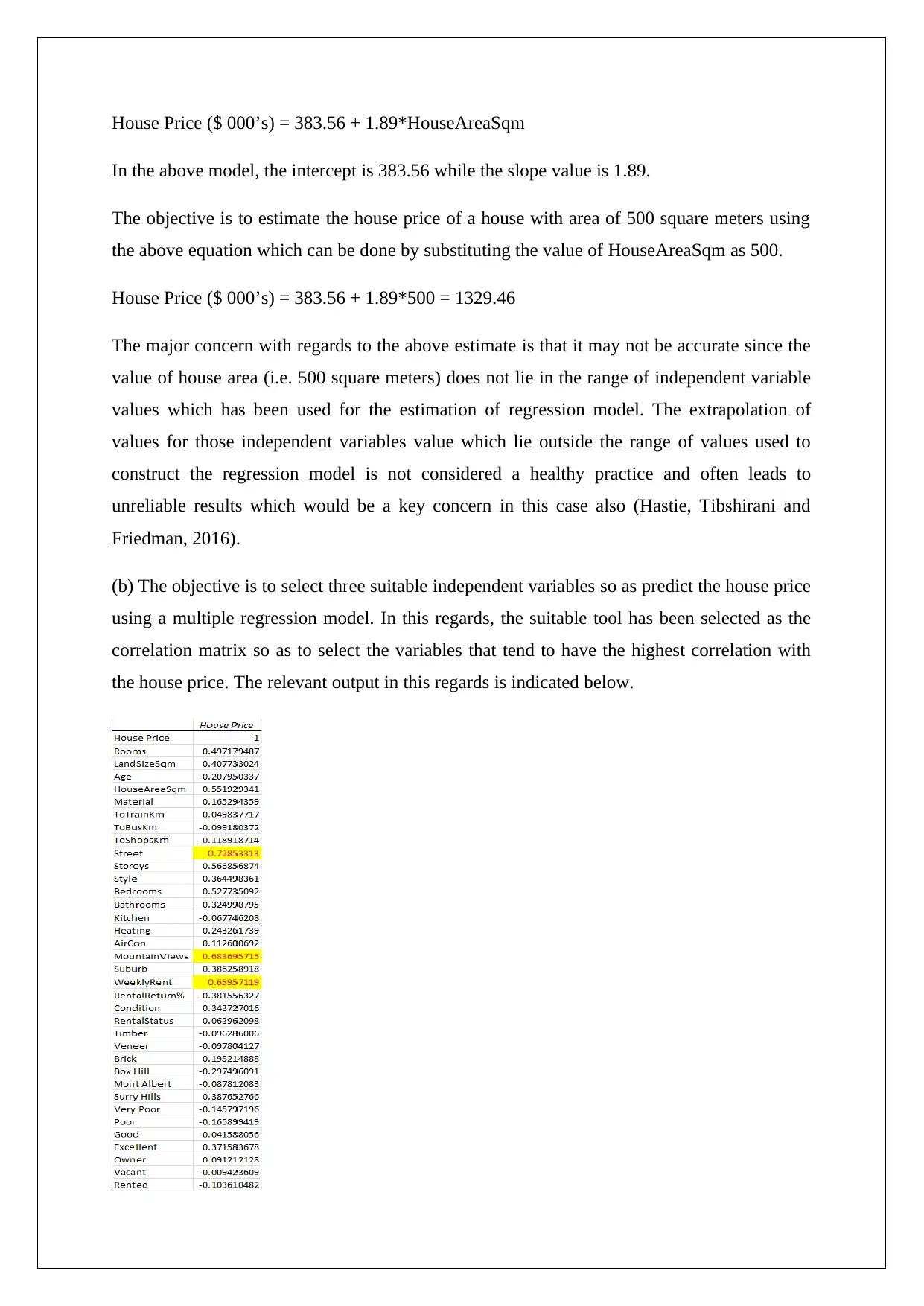
(b) The objective is to select three suitable independent variables so as predict the house price
using a multiple regression model. In this regards, the suitable tool has been selected as the
correlation matrix so as to select the variables that tend to have the highest correlation with
the house price. The relevant output in this regards is indicated below.

From the above output, it is apparent that the three variables having the highest correlation
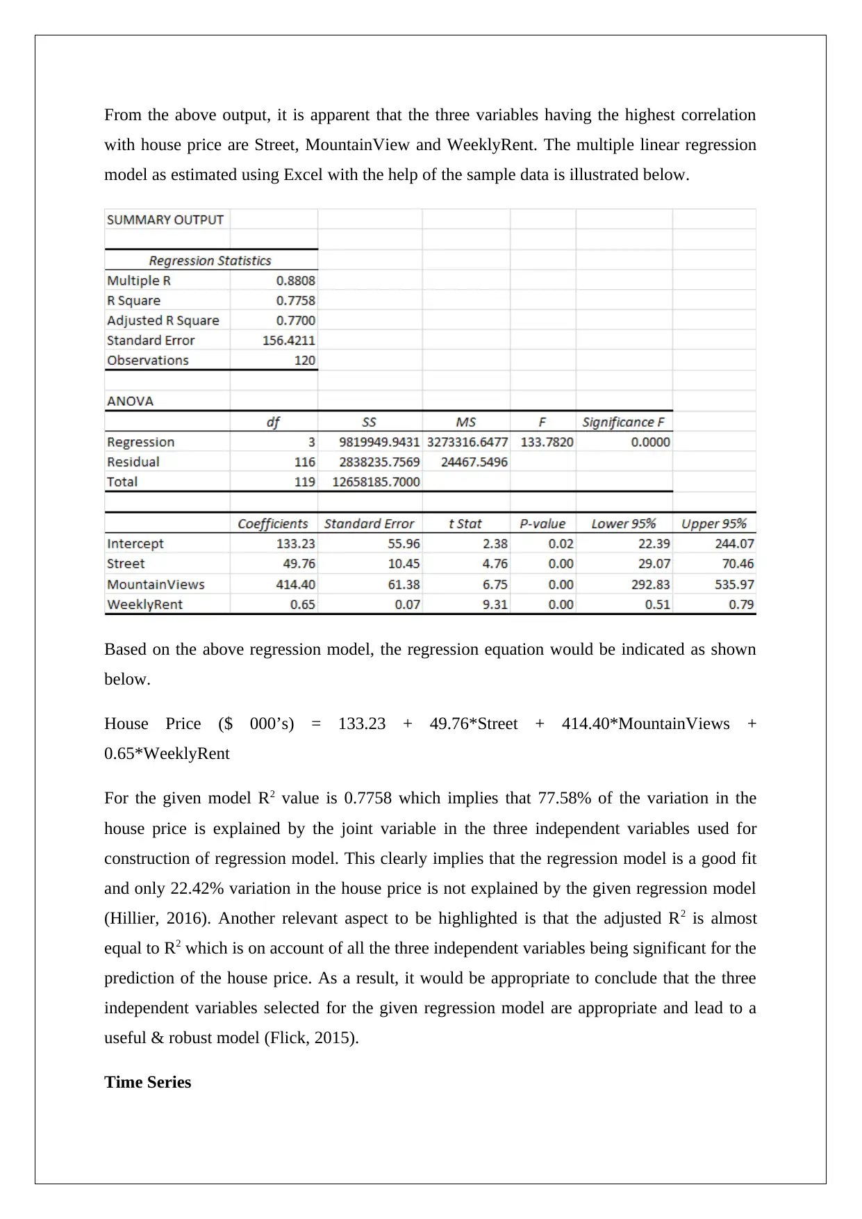
with house price are Street, MountainView and WeeklyRent. The multiple linear regression
model as estimated using Excel with the help of the sample data is illustrated below.
Based on the above regression model, the regression equation would be indicated as shown
below.
House Price ($ 000’s) = 133.23 + 49.76*Street + 414.40*MountainViews +
0.65*WeeklyRent
For the given model R2 value is 0.7758 which implies that 77.58% of the variation in the
house price is explained by the joint variable in the three independent variables used for
construction of regression model. This clearly implies that the regression model is a good fit
and only 22.42% variation in the house price is not explained by the given regression model
(Hillier, 2016). Another relevant aspect to be highlighted is that the adjusted R2 is almost
equal to R2 which is on account of all the three independent variables being significant for the
prediction of the house price. As a result, it would be appropriate to conclude that the three
independent variables selected for the given regression model are appropriate and lead to a
useful & robust model (Flick, 2015).
Time Series

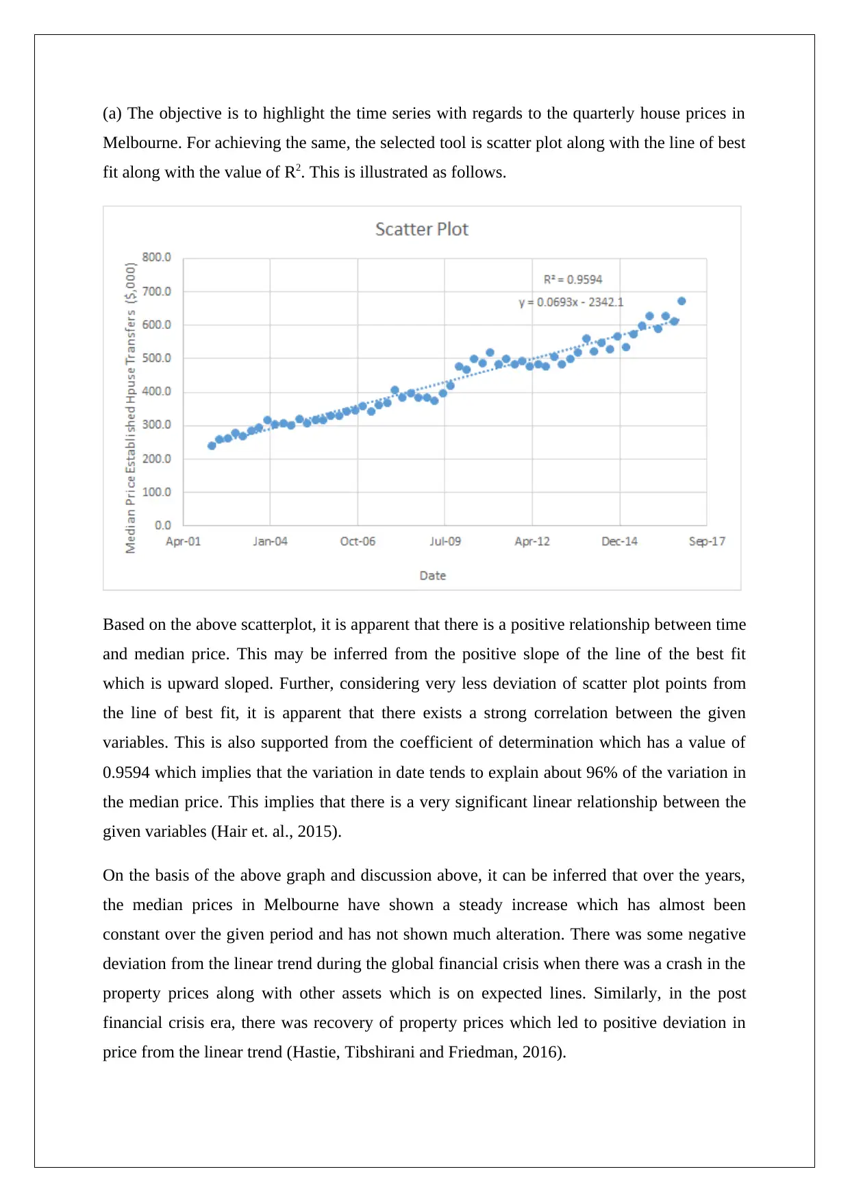
(a) The objective is to highlight the time series with regards to the quarterly house prices in
Melbourne. For achieving the same, the selected tool is scatter plot along with the line of best
fit along with the value of R2. This is illustrated as follows.
Based on the above scatterplot, it is apparent that there is a positive relationship between time
and median price. This may be inferred from the positive slope of the line of the best fit
which is upward sloped. Further, considering very less deviation of scatter plot points from
the line of best fit, it is apparent that there exists a strong correlation between the given
variables. This is also supported from the coefficient of determination which has a value of
0.9594 which implies that the variation in date tends to explain about 96% of the variation in
the median price. This implies that there is a very significant linear relationship between the
given variables (Hair et. al., 2015).
On the basis of the above graph and discussion above, it can be inferred that over the years,
the median prices in Melbourne have shown a steady increase which has almost been
constant over the given period and has not shown much alteration. There was some negative
deviation from the linear trend during the global financial crisis when there was a crash in the
property prices along with other assets which is on expected lines. Similarly, in the post
financial crisis era, there was recovery of property prices which led to positive deviation in
price from the linear trend (Hastie, Tibshirani and Friedman, 2016).

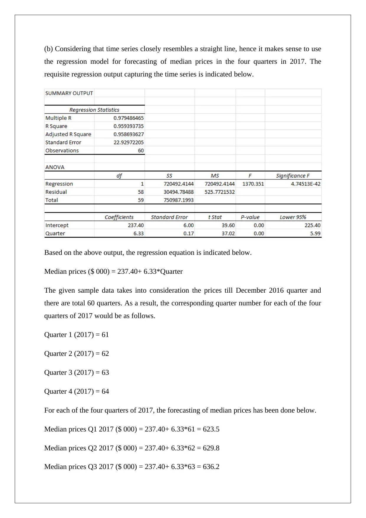
(b) Considering that time series closely resembles a straight line, hence it makes sense to use
the regression model for forecasting of median prices in the four quarters in 2017. The
requisite regression output capturing the time series is indicated below.
Based on the above output, the regression equation is indicated below.
Median prices ($ 000) = 237.40+ 6.33*Quarter
The given sample data takes into consideration the prices till December 2016 quarter and
there are total 60 quarters. As a result, the corresponding quarter number for each of the four
quarters of 2017 would be as follows.
Quarter 1 (2017) = 61
Quarter 2 (2017) = 62
Quarter 3 (2017) = 63
Quarter 4 (2017) = 64
For each of the four quarters of 2017, the forecasting of median prices has been done below.
Median prices Q1 2017 ($ 000) = 237.40+ 6.33*61 = 623.5
Median prices Q2 2017 ($ 000) = 237.40+ 6.33*62 = 629.8
Median prices Q3 2017 ($ 000) = 237.40+ 6.33*63 = 636.2

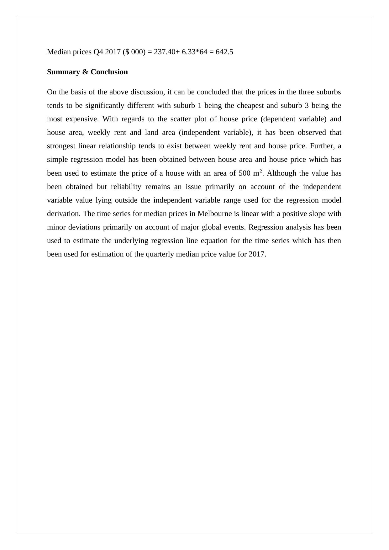
Median prices Q4 2017 ($ 000) = 237.40+ 6.33*64 = 642.5
Summary & Conclusion
On the basis of the above discussion, it can be concluded that the prices in the three suburbs
tends to be significantly different with suburb 1 being the cheapest and suburb 3 being the
most expensive. With regards to the scatter plot of house price (dependent variable) and
house area, weekly rent and land area (independent variable), it has been observed that
strongest linear relationship tends to exist between weekly rent and house price. Further, a
simple regression model has been obtained between house area and house price which has
been used to estimate the price of a house with an area of 500 m2. Although the value has
been obtained but reliability remains an issue primarily on account of the independent
variable value lying outside the independent variable range used for the regression model
derivation. The time series for median prices in Melbourne is linear with a positive slope with
minor deviations primarily on account of major global events. Regression analysis has been
used to estimate the underlying regression line equation for the time series which has then
been used for estimation of the quarterly median price value for 2017.

References
Eriksson, P. and Kovalainen, A. (2015). Quantitative methods in business research (3rd ed.).
London: Sage Publications.
Flick, U. (2015). Introducing research methodology: A beginner's guide to doing a research
project (4th ed.). New York: Sage Publications.
Hair, J. F., Wolfinbarger, M., Money, A. H., Samouel, P., and Page, M. J. (2015). Essentials
of business research methods (2nd ed.). New York: Routledge.
Hastie, T., Tibshirani, R. and Friedman, J. (2016). The Elements of Statistical Learning (4th
ed.). New York: Springer Publications.
Hillier, F. (2016). Introduction to Operations Research. (6th ed.). New York: McGraw Hill
Publications.
Lieberman, F. J., Nag, B., Hiller, F.S. and Basu, P. (2013) Introduction To Operations
Research. (5th ed.) New Delhi: Tata McGraw Hill Publishers.
Medhi, J. (2016) Statistical Methods: An Introductory Text. (4th ed.) Sydney: New Age
International.