Statistical Report: Correlation, Regression, Time Series Analysis
VerifiedAdded on 2023/04/21
|12
|2356
|92
Report
AI Summary
This report uses various statistical methods, including correlation and regression analysis, to analyze sample data and draw estimations about the population, with a focus on house prices in Melbourne. It investigates the relationship between house prices and suburbs, as well as the correlation between house prices and independent variables like land size, house area, and weekly rent. Regression analysis is applied to determine the relationship between house area and house price, and a multiple regression model is used to identify the most satisfactory explanatory variables. Time series analysis is performed on Melbourne house prices to forecast future values. The report concludes that weekly rent has the strongest association with house prices and that the time series analysis indicates an increasing trend in Melbourne median house prices over time. Desklib offers a wealth of similar solved assignments and study resources for students.
FOUNDATION SKILLS IN DATA ANALYSIS
STUDENT ID:
[Pick the date]
STUDENT ID:
[Pick the date]
Paraphrase This Document
Need a fresh take? Get an instant paraphrase of this document with our AI Paraphraser
Introduction
Various statistical methods have been taken into consideration in order to analyse the sample
data so as to draw estimation about the population and to summarise the given data to make
relevant conclusion. In present scenario, descriptive statistics techniques have been used to
summarise the data. The main aim of the statistical report is to apply correlation and
regression analysis technique so that the sample can be analysed and requisite conclusions
can be made. The association among the relevant dependent and independent variables would
also be drawn so that the most satisfactory explanatory variables can be found that shows
highest level of correlation with the dependent variable. The time series analysis has also be
performed for the median price of houses in Melbourne data set.
Relationships
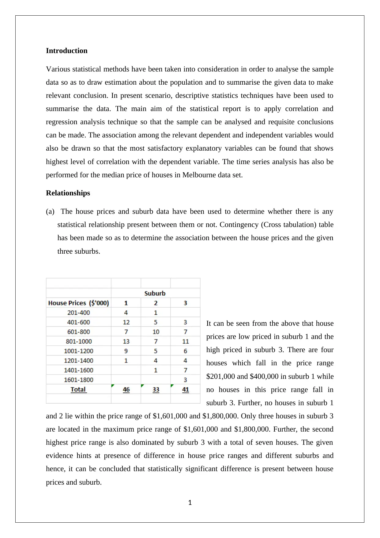
(a) The house prices and suburb data have been used to determine whether there is any
statistical relationship present between them or not. Contingency (Cross tabulation) table
has been made so as to determine the association between the house prices and the given
three suburbs.
It can be seen from the above that house
prices are low priced in suburb 1 and the
high priced in suburb 3. There are four
houses which fall in the price range
$201,000 and $400,000 in suburb 1 while
no houses in this price range fall in
suburb 3. Further, no houses in suburb 1
and 2 lie within the price range of $1,601,000 and $1,800,000. Only three houses in suburb 3
are located in the maximum price range of $1,601,000 and $1,800,000. Further, the second
highest price range is also dominated by suburb 3 with a total of seven houses. The given
evidence hints at presence of difference in house price ranges and different suburbs and
hence, it can be concluded that statistically significant difference is present between house
prices and suburb.
1
Various statistical methods have been taken into consideration in order to analyse the sample
data so as to draw estimation about the population and to summarise the given data to make
relevant conclusion. In present scenario, descriptive statistics techniques have been used to
summarise the data. The main aim of the statistical report is to apply correlation and
regression analysis technique so that the sample can be analysed and requisite conclusions
can be made. The association among the relevant dependent and independent variables would
also be drawn so that the most satisfactory explanatory variables can be found that shows
highest level of correlation with the dependent variable. The time series analysis has also be
performed for the median price of houses in Melbourne data set.
Relationships
(a) The house prices and suburb data have been used to determine whether there is any
statistical relationship present between them or not. Contingency (Cross tabulation) table
has been made so as to determine the association between the house prices and the given
three suburbs.
It can be seen from the above that house
prices are low priced in suburb 1 and the
high priced in suburb 3. There are four
houses which fall in the price range
$201,000 and $400,000 in suburb 1 while
no houses in this price range fall in
suburb 3. Further, no houses in suburb 1
and 2 lie within the price range of $1,601,000 and $1,800,000. Only three houses in suburb 3
are located in the maximum price range of $1,601,000 and $1,800,000. Further, the second
highest price range is also dominated by suburb 3 with a total of seven houses. The given
evidence hints at presence of difference in house price ranges and different suburbs and
hence, it can be concluded that statistically significant difference is present between house
prices and suburb.
1
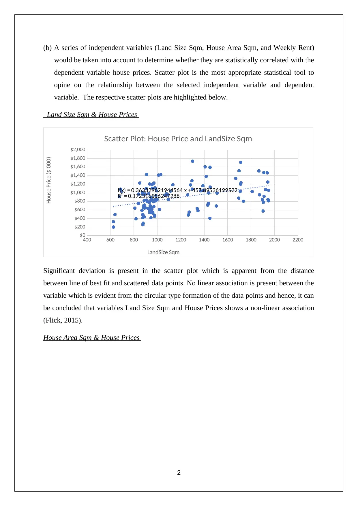
(b) A series of independent variables (Land Size Sqm, House Area Sqm, and Weekly Rent)
would be taken into account to determine whether they are statistically correlated with the
dependent variable house prices. Scatter plot is the most appropriate statistical tool to
opine on the relationship between the selected independent variable and dependent
variable. The respective scatter plots are highlighted below.
Land Size Sqm & House Prices
400 600 800 1000 1200 1400 1600 1800 2000 2200
$0
$200
$400
$600
$800
$1,000
$1,200
$1,400
$1,600
$1,800
$2,000
f(x) = 0.363329621944564 x + 457.89536199522
R² = 0.172316556247288
Scatter Plot: House Price and LandSize Sqm
LandSize Sqm
House Price ($'000)
Significant deviation is present in the scatter plot which is apparent from the distance
between line of best fit and scattered data points. No linear association is present between the
variable which is evident from the circular type formation of the data points and hence, it can
be concluded that variables Land Size Sqm and House Prices shows a non-linear association
(Flick, 2015).
House Area Sqm & House Prices
2
⊘ This is a preview!⊘
Do you want full access?
Subscribe today to unlock all pages.
Trusted by 1+ million students worldwide
100 150 200 250 300 350 400 450 500
$0
$200
$400
$600
$800
$1,000
$1,200
$1,400
$1,600
$1,800
$2,000
f(x) = 1.93409920082195 x + 370.011106927843
R² = 0.318008119408161
Scatter Plot: House Price snd House Area Sqm
House Area Sqm
House Price ($'000)
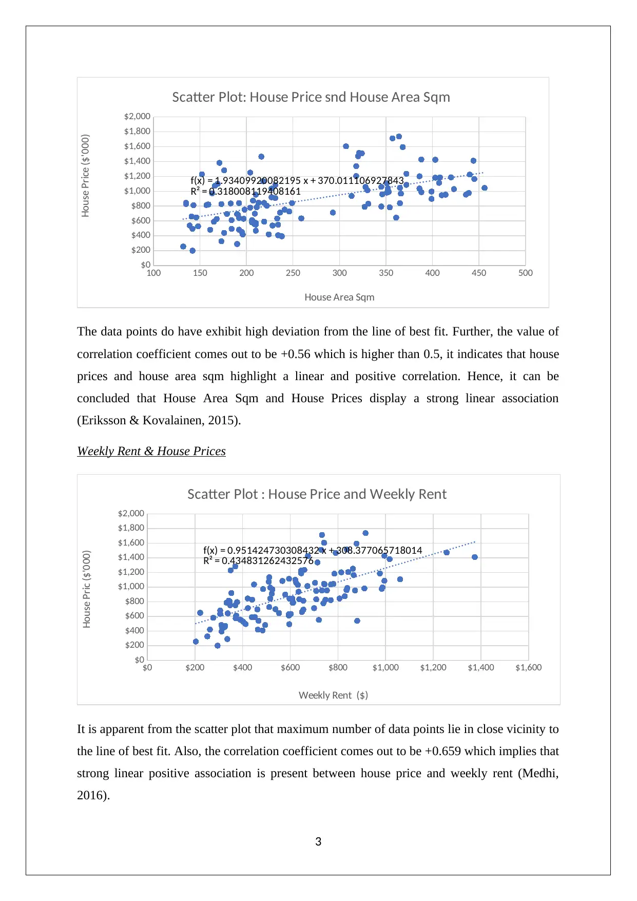
The data points do have exhibit high deviation from the line of best fit. Further, the value of
correlation coefficient comes out to be +0.56 which is higher than 0.5, it indicates that house
prices and house area sqm highlight a linear and positive correlation. Hence, it can be
concluded that House Area Sqm and House Prices display a strong linear association
(Eriksson & Kovalainen, 2015).
Weekly Rent & House Prices
$0 $200 $400 $600 $800 $1,000 $1,200 $1,400 $1,600
$0
$200
$400
$600
$800
$1,000
$1,200
$1,400
$1,600
$1,800
$2,000
f(x) = 0.951424730308432 x + 308.377065718014
R² = 0.434831262432576
Scatter Plot : House Price and Weekly Rent
Weekly Rent ($)
House Pric ($'000)
It is apparent from the scatter plot that maximum number of data points lie in close vicinity to
the line of best fit. Also, the correlation coefficient comes out to be +0.659 which implies that
strong linear positive association is present between house price and weekly rent (Medhi,
2016).
3
$0
$200
$400
$600
$800
$1,000
$1,200
$1,400
$1,600
$1,800
$2,000
f(x) = 1.93409920082195 x + 370.011106927843
R² = 0.318008119408161
Scatter Plot: House Price snd House Area Sqm
House Area Sqm
House Price ($'000)
The data points do have exhibit high deviation from the line of best fit. Further, the value of
correlation coefficient comes out to be +0.56 which is higher than 0.5, it indicates that house
prices and house area sqm highlight a linear and positive correlation. Hence, it can be
concluded that House Area Sqm and House Prices display a strong linear association
(Eriksson & Kovalainen, 2015).
Weekly Rent & House Prices
$0 $200 $400 $600 $800 $1,000 $1,200 $1,400 $1,600
$0
$200
$400
$600
$800
$1,000
$1,200
$1,400
$1,600
$1,800
$2,000
f(x) = 0.951424730308432 x + 308.377065718014
R² = 0.434831262432576
Scatter Plot : House Price and Weekly Rent
Weekly Rent ($)
House Pric ($'000)
It is apparent from the scatter plot that maximum number of data points lie in close vicinity to
the line of best fit. Also, the correlation coefficient comes out to be +0.659 which implies that
strong linear positive association is present between house price and weekly rent (Medhi,
2016).
3
Paraphrase This Document
Need a fresh take? Get an instant paraphrase of this document with our AI Paraphraser
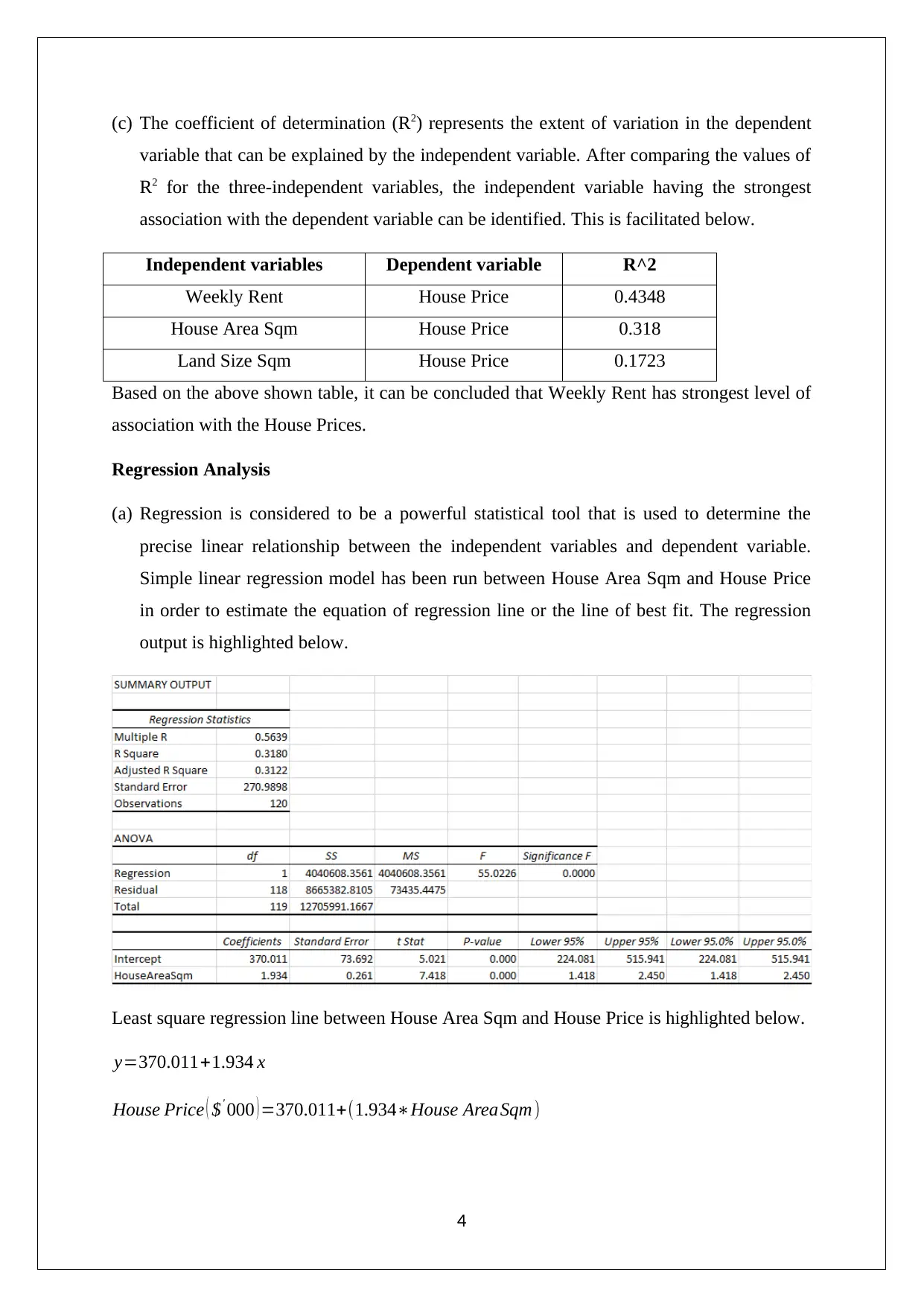
(c) The coefficient of determination (R2) represents the extent of variation in the dependent
variable that can be explained by the independent variable. After comparing the values of
R2 for the three-independent variables, the independent variable having the strongest
association with the dependent variable can be identified. This is facilitated below.
Independent variables Dependent variable R^2
Weekly Rent House Price 0.4348
House Area Sqm House Price 0.318
Land Size Sqm House Price 0.1723
Based on the above shown table, it can be concluded that Weekly Rent has strongest level of
association with the House Prices.
Regression Analysis
(a) Regression is considered to be a powerful statistical tool that is used to determine the
precise linear relationship between the independent variables and dependent variable.
Simple linear regression model has been run between House Area Sqm and House Price
in order to estimate the equation of regression line or the line of best fit. The regression
output is highlighted below.
Least square regression line between House Area Sqm and House Price is highlighted below.
y=370.011+1.934 x
House Price ( $' 000 ) =370.011+(1.934∗House Area Sqm)
4
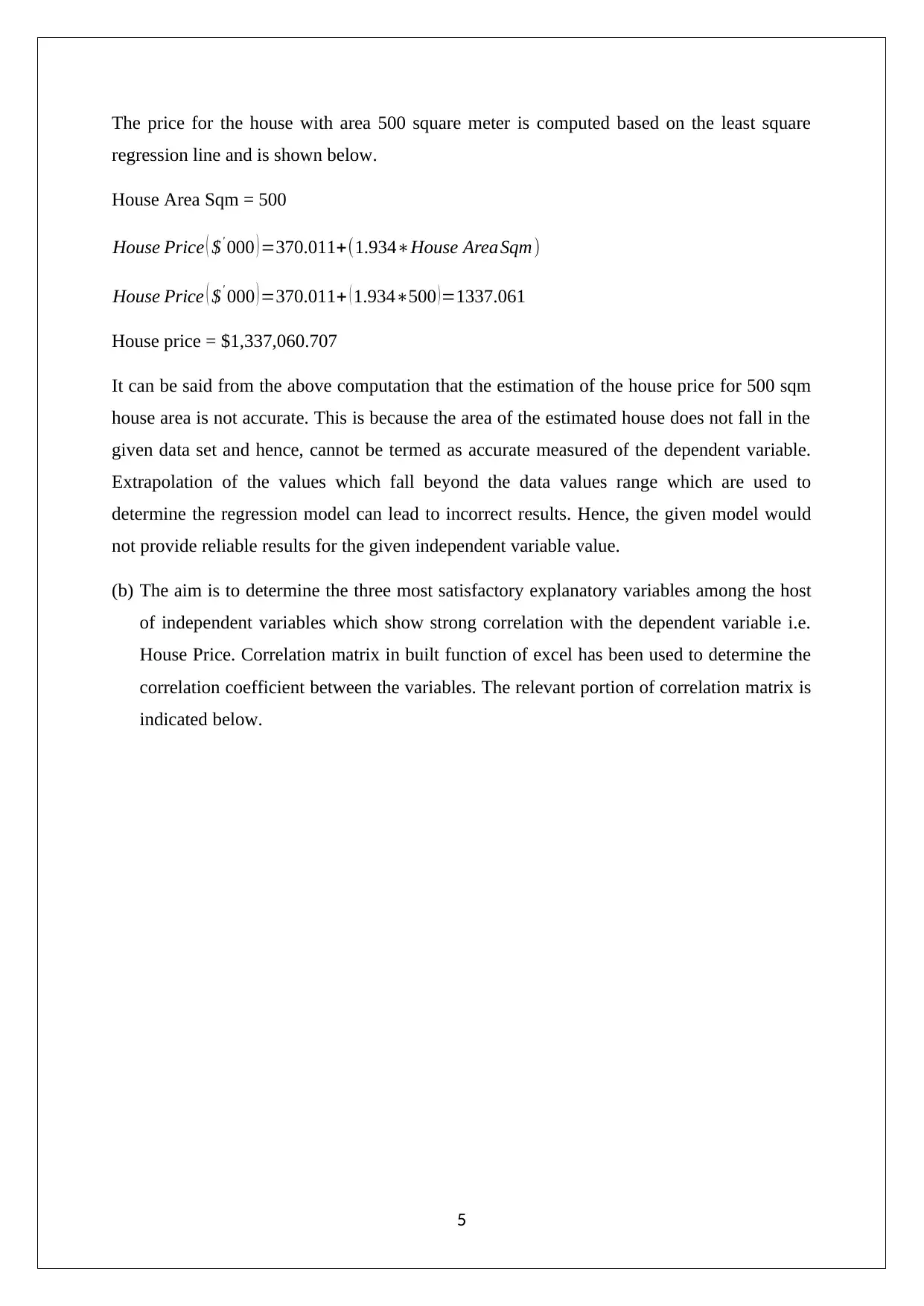
The price for the house with area 500 square meter is computed based on the least square
regression line and is shown below.
House Area Sqm = 500
House Price ( $' 000 ) =370.011+(1.934∗House Area Sqm)
House Price ( $' 000 ) =370.011+ ( 1.934∗500 ) =1337.061
House price = $1,337,060.707
It can be said from the above computation that the estimation of the house price for 500 sqm
house area is not accurate. This is because the area of the estimated house does not fall in the
given data set and hence, cannot be termed as accurate measured of the dependent variable.
Extrapolation of the values which fall beyond the data values range which are used to
determine the regression model can lead to incorrect results. Hence, the given model would
not provide reliable results for the given independent variable value.
(b) The aim is to determine the three most satisfactory explanatory variables among the host
of independent variables which show strong correlation with the dependent variable i.e.
House Price. Correlation matrix in built function of excel has been used to determine the
correlation coefficient between the variables. The relevant portion of correlation matrix is
indicated below.
5
⊘ This is a preview!⊘
Do you want full access?
Subscribe today to unlock all pages.
Trusted by 1+ million students worldwide
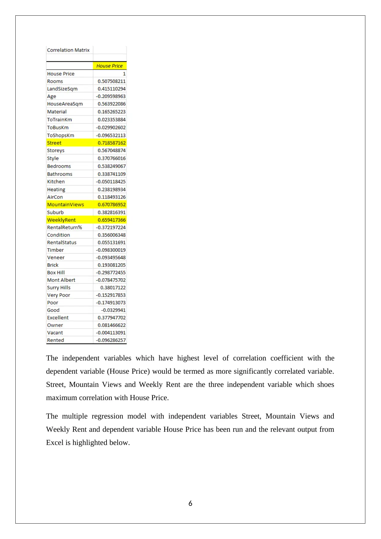
The independent variables which have highest level of correlation coefficient with the
dependent variable (House Price) would be termed as more significantly correlated variable.
Street, Mountain Views and Weekly Rent are the three independent variable which shoes
maximum correlation with House Price.
The multiple regression model with independent variables Street, Mountain Views and
Weekly Rent and dependent variable House Price has been run and the relevant output from
Excel is highlighted below.
6
Paraphrase This Document
Need a fresh take? Get an instant paraphrase of this document with our AI Paraphraser
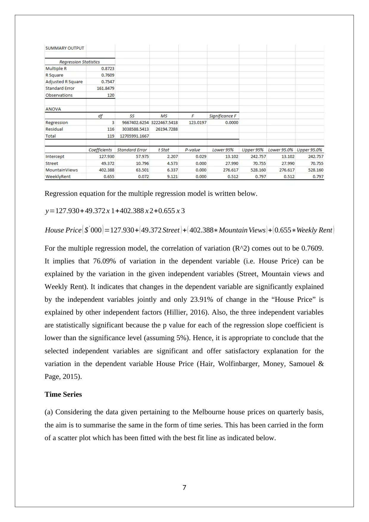
Regression equation for the multiple regression model is written below.
y=127.930+ 49.372 x 1+402.388 x 2+0.655 x 3
House Price ( $' 000 ) =127.930+ ( 49.372 Street ) + ( 402.388∗Mountain Views ) + ( 0.655∗Weekly Rent )
For the multiple regression model, the correlation of variation (R^2) comes out to be 0.7609.
It implies that 76.09% of variation in the dependent variable (i.e. House Price) can be
explained by the variation in the given independent variables (Street, Mountain views and
Weekly Rent). It indicates that changes in the dependent variable are significantly explained
by the independent variables jointly and only 23.91% of change in the “House Price” is
explained by other independent factors (Hillier, 2016). Also, the three independent variables
are statistically significant because the p value for each of the regression slope coefficient is
lower than the significance level (assuming 5%). Hence, it is appropriate to conclude that the
selected independent variables are significant and offer satisfactory explanation for the
variation in the dependent variable House Price (Hair, Wolfinbarger, Money, Samouel &
Page, 2015).
Time Series
(a) Considering the data given pertaining to the Melbourne house prices on quarterly basis,
the aim is to summarise the same in the form of time series. This has been carried in the form
of a scatter plot which has been fitted with the best fit line as indicated below.
7
Apr-01 Jan-04 Oct-06 Jul-09 Apr-12 Dec-14 Sep-17
0.0
100.0
200.0
300.0
400.0
500.0
600.0
700.0
800.0
f(x) = 0.0692940701190254 x − 2342.10181013878
R² = 0.959410047154515
Scatter Plot: Median Price of established house transfer
melbourne
Date
Median Price of established houe transfer
Melbourne ($'000)
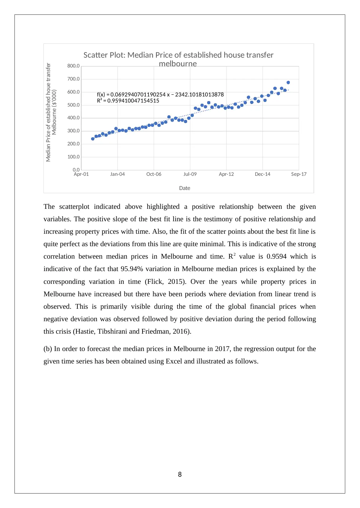
The scatterplot indicated above highlighted a positive relationship between the given
variables. The positive slope of the best fit line is the testimony of positive relationship and
increasing property prices with time. Also, the fit of the scatter points about the best fit line is
quite perfect as the deviations from this line are quite minimal. This is indicative of the strong
correlation between median prices in Melbourne and time. R2 value is 0.9594 which is
indicative of the fact that 95.94% variation in Melbourne median prices is explained by the
corresponding variation in time (Flick, 2015). Over the years while property prices in
Melbourne have increased but there have been periods where deviation from linear trend is
observed. This is primarily visible during the time of the global financial prices when
negative deviation was observed followed by positive deviation during the period following
this crisis (Hastie, Tibshirani and Friedman, 2016).
(b) In order to forecast the median prices in Melbourne in 2017, the regression output for the
given time series has been obtained using Excel and illustrated as follows.
8
0.0
100.0
200.0
300.0
400.0
500.0
600.0
700.0
800.0
f(x) = 0.0692940701190254 x − 2342.10181013878
R² = 0.959410047154515
Scatter Plot: Median Price of established house transfer
melbourne
Date
Median Price of established houe transfer
Melbourne ($'000)
The scatterplot indicated above highlighted a positive relationship between the given
variables. The positive slope of the best fit line is the testimony of positive relationship and
increasing property prices with time. Also, the fit of the scatter points about the best fit line is
quite perfect as the deviations from this line are quite minimal. This is indicative of the strong
correlation between median prices in Melbourne and time. R2 value is 0.9594 which is
indicative of the fact that 95.94% variation in Melbourne median prices is explained by the
corresponding variation in time (Flick, 2015). Over the years while property prices in
Melbourne have increased but there have been periods where deviation from linear trend is
observed. This is primarily visible during the time of the global financial prices when
negative deviation was observed followed by positive deviation during the period following
this crisis (Hastie, Tibshirani and Friedman, 2016).
(b) In order to forecast the median prices in Melbourne in 2017, the regression output for the
given time series has been obtained using Excel and illustrated as follows.
8
⊘ This is a preview!⊘
Do you want full access?
Subscribe today to unlock all pages.
Trusted by 1+ million students worldwide
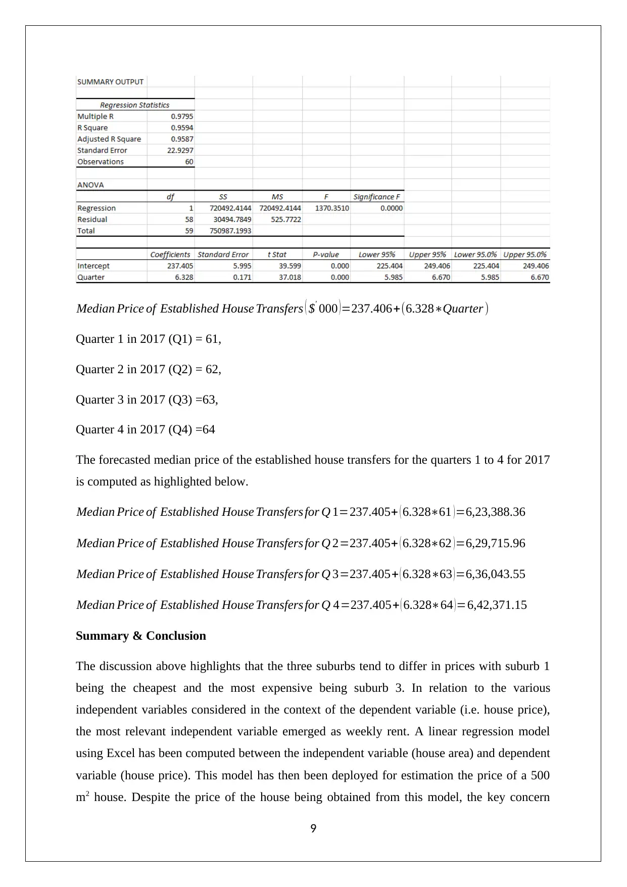
Median Price of Established House Transfers ( $' 000 )=237.406+(6.328∗Quarter )
Quarter 1 in 2017 (Q1) = 61,
Quarter 2 in 2017 (Q2) = 62,
Quarter 3 in 2017 (Q3) =63,
Quarter 4 in 2017 (Q4) =64
The forecasted median price of the established house transfers for the quarters 1 to 4 for 2017
is computed as highlighted below.
Median Price of Established House Transfers for Q 1=237.405+ ( 6.328∗61 )=6,23,388.36
Median Price of Established House Transfers for Q 2=237.405+ ( 6.328∗62 )=6,29,715.96
Median Price of Established House Transfers for Q 3=237.405+ ( 6.328∗63 )=6,36,043.55
Median Price of Established House Transfers for Q 4=237.405+ ( 6.328∗64 )=6,42,371.15
Summary & Conclusion
The discussion above highlights that the three suburbs tend to differ in prices with suburb 1
being the cheapest and the most expensive being suburb 3. In relation to the various
independent variables considered in the context of the dependent variable (i.e. house price),
the most relevant independent variable emerged as weekly rent. A linear regression model
using Excel has been computed between the independent variable (house area) and dependent
variable (house price). This model has then been deployed for estimation the price of a 500
m2 house. Despite the price of the house being obtained from this model, the key concern
9
Paraphrase This Document
Need a fresh take? Get an instant paraphrase of this document with our AI Paraphraser
remained as reliability since the independent variable value is not included in the set of
values used in computation of regression model. The Melbourne median prices have
increased over the years which are captured by the positive slope of the time series. Further,
the regression model has been predicted for the Melbourne median prices so as to assist in the
determination of 2017 quarterly Melbourne median prices.
References
Eriksson, P. & Kovalainen, A. (2015). Quantitative methods in business research (3rd ed.).
London: Sage Publications.
10
Flick, U. (2015). Introducing research methodology: A beginner's guide to doing a research
project (4th ed.). New York: Sage Publications.
Hair, J. F., Wolfinbarger, M., Money, A. H., Samouel, P., & Page, M. J. (2015). Essentials of
business research methods (2nd ed.). New York: Routledge.
Hastie, T., Tibshirani, R. & Friedman, J. (2016). The Elements of Statistical Learning (4th
ed.). New York: Springer Publications.
Hillier, F. (2016). Introduction to Operations Research. (6th ed.). New York: McGraw Hill
Publications.
Medhi, J. (2016) Statistical Methods: An Introductory Text. (4th ed.) Sydney: New Age
International.
11
⊘ This is a preview!⊘
Do you want full access?
Subscribe today to unlock all pages.
Trusted by 1+ million students worldwide
1 out of 12
Related Documents


Your All-in-One AI-Powered Toolkit for Academic Success.
+13062052269
info@desklib.com
Available 24*7 on WhatsApp / Email
![[object Object]](/_next/static/media/star-bottom.7253800d.svg)
Unlock your academic potential
Copyright © 2020–2025 A2Z Services. All Rights Reserved. Developed and managed by ZUCOL.