Frequency Distribution - PDF

STATISTICS
Student Name
[Pick the date]

Question 1
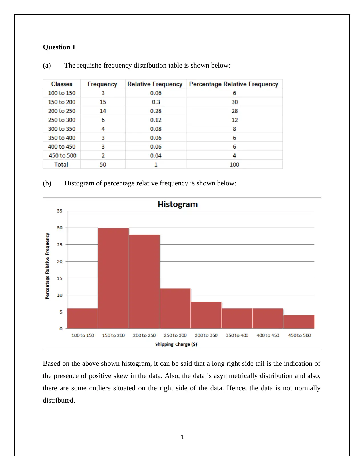
(a) The requisite frequency distribution table is shown below:
(b) Histogram of percentage relative frequency is shown below:
Based on the above shown histogram, it can be said that a long right side tail is the indication of
the presence of positive skew in the data. Also, the data is asymmetrically distribution and also,
there are some outliers situated on the right side of the data. Hence, the data is not normally
distributed.
1

(c) Considering the asymmetric shape of the graph and the potential presence of outliers, it
would be recommended to use median as the preferred indicator of location and not
mean. The mean in such cases can be skewed owing to present of high values and hence
may represent an exaggerated indication of central location.
Question 2
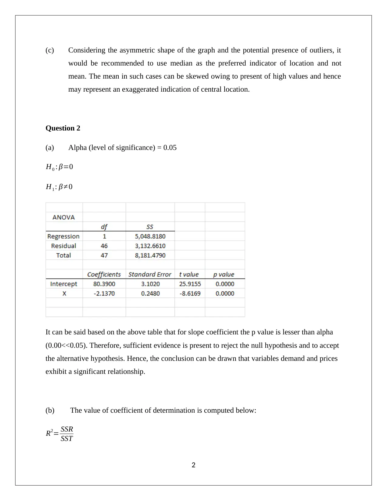
(a) Alpha (level of significance) = 0.05
H0 : β=0
H1 : β ≠ 0
It can be said based on the above table that for slope coefficient the p value is lesser than alpha
(0.00<<0.05). Therefore, sufficient evidence is present to reject the null hypothesis and to accept
the alternative hypothesis. Hence, the conclusion can be drawn that variables demand and prices
exhibit a significant relationship.
(b) The value of coefficient of determination is computed below:
R2= SSR
SST
2

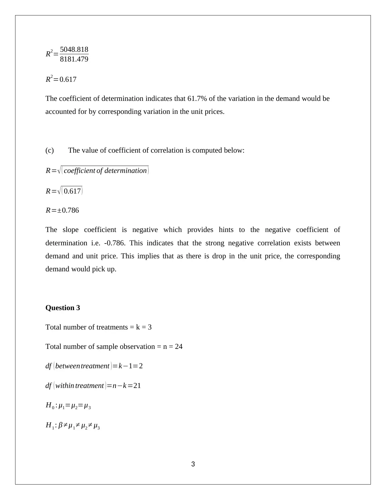
R2= 5048.818
8181.479
R2=0.617
The coefficient of determination indicates that 61.7% of the variation in the demand would be
accounted for by corresponding variation in the unit prices.
(c) The value of coefficient of correlation is computed below:
R= √ ( coefficient of determination )
R= √ ( 0.617 )
R=±0.786
The slope coefficient is negative which provides hints to the negative coefficient of
determination i.e. -0.786. This indicates that the strong negative correlation exists between
demand and unit price. This implies that as there is drop in the unit price, the corresponding
demand would pick up.
Question 3
Total number of treatments = k = 3
Total number of sample observation = n = 24
df ( between treatment )=k−1=2
df ( within treatment ) =n−k =21
H0 : μ1=μ2=μ3
H1 : β ≠ μ1 ≠ μ2 ≠ μ3
3

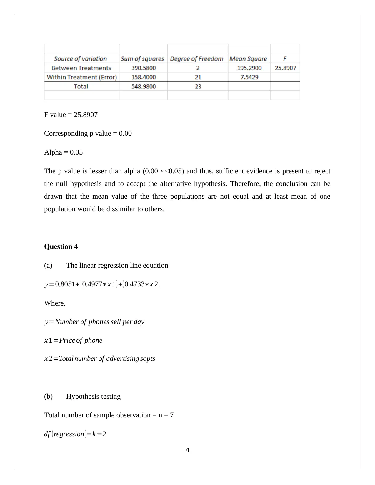
F value = 25.8907
Corresponding p value = 0.00
Alpha = 0.05
The p value is lesser than alpha (0.00 <<0.05) and thus, sufficient evidence is present to reject
the null hypothesis and to accept the alternative hypothesis. Therefore, the conclusion can be
drawn that the mean value of the three populations are not equal and at least mean of one
population would be dissimilar to others.
Question 4
(a) The linear regression line equation
y=0.8051+ ( 0.4977∗x 1 ) + ( 0.4733∗x 2 )
Where,
y=Number of phones sell per day
x 1=Price of phone
x 2=Total number of advertising sopts
(b) Hypothesis testing
Total number of sample observation = n = 7
df ( regression ) =k =2
4

df ( residual ) =n−k−1=4
H0 : β1=β2=β3=… … … . βn=0
H1 : At least one β ≠ 0
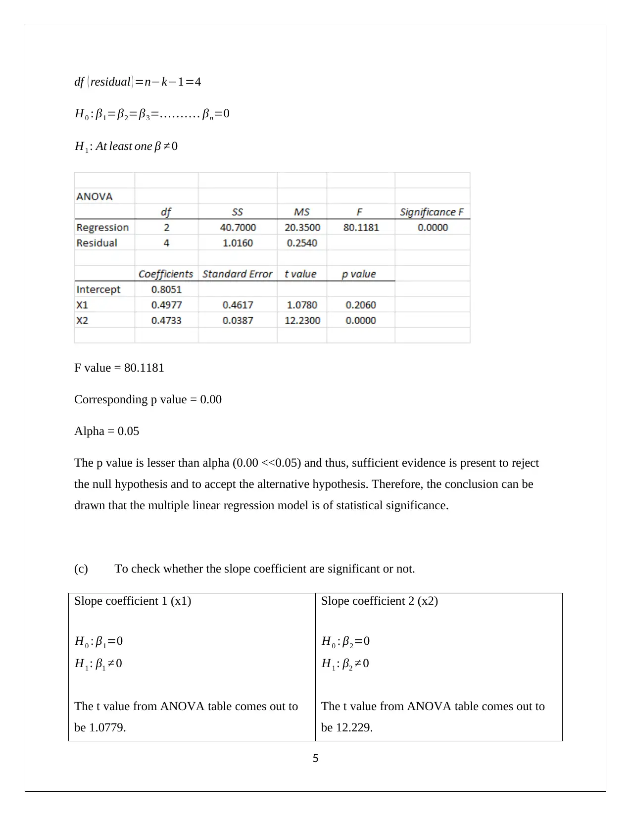
F value = 80.1181
Corresponding p value = 0.00
Alpha = 0.05
The p value is lesser than alpha (0.00 <<0.05) and thus, sufficient evidence is present to reject
the null hypothesis and to accept the alternative hypothesis. Therefore, the conclusion can be
drawn that the multiple linear regression model is of statistical significance.
(c) To check whether the slope coefficient are significant or not.
Slope coefficient 1 (x1)
H0 : β1=0
H1 : β1 ≠ 0
The t value from ANOVA table comes out to
be 1.0779.
Slope coefficient 2 (x2)
H0 : β2=0
H1 : β2 ≠ 0
The t value from ANOVA table comes out to
be 12.229.
5

The p value corresponding to degree of
freedom and above t value comes out to be
0.206.
Level of significance = 0.05
The p value is greater than level of significance
and therefore, insufficient evidence presents to
reject the null hypothesis.
The conclusion can be made that mobile phone
prices is not a significant variable.
The p value corresponding to degree of
freedom and above t value comes out to be
0.000.
Level of significance = 0.05
The p value is lesser than level of significance
and therefore, sufficient evidence presents to
reject the null hypothesis and to accept
alternative hypothesis.
The conclusion can be made that advertising
spots is a significant variable.
(d) The value of slope coefficient of variable x2 comes out to be 0.4733.
This value indicates that when the number of advertising spots for mobile phone is increased by
one unit, then the respective per day sale would also be increased by 0.4733 units.
(e) Per day sale =?
Total number of advertising spots made for mobile phones (x2) = 10
Price for the mobile phone (x1) = $20,000
Hence,
Regression equation
y=0.8051+ ( 0.4977∗x 1 ) + ( 0.4733∗x 2 )
y=0.8051+ { ( 0.4977∗20000 ) } + { ( 0.4733∗10 ) }
6

y=9960
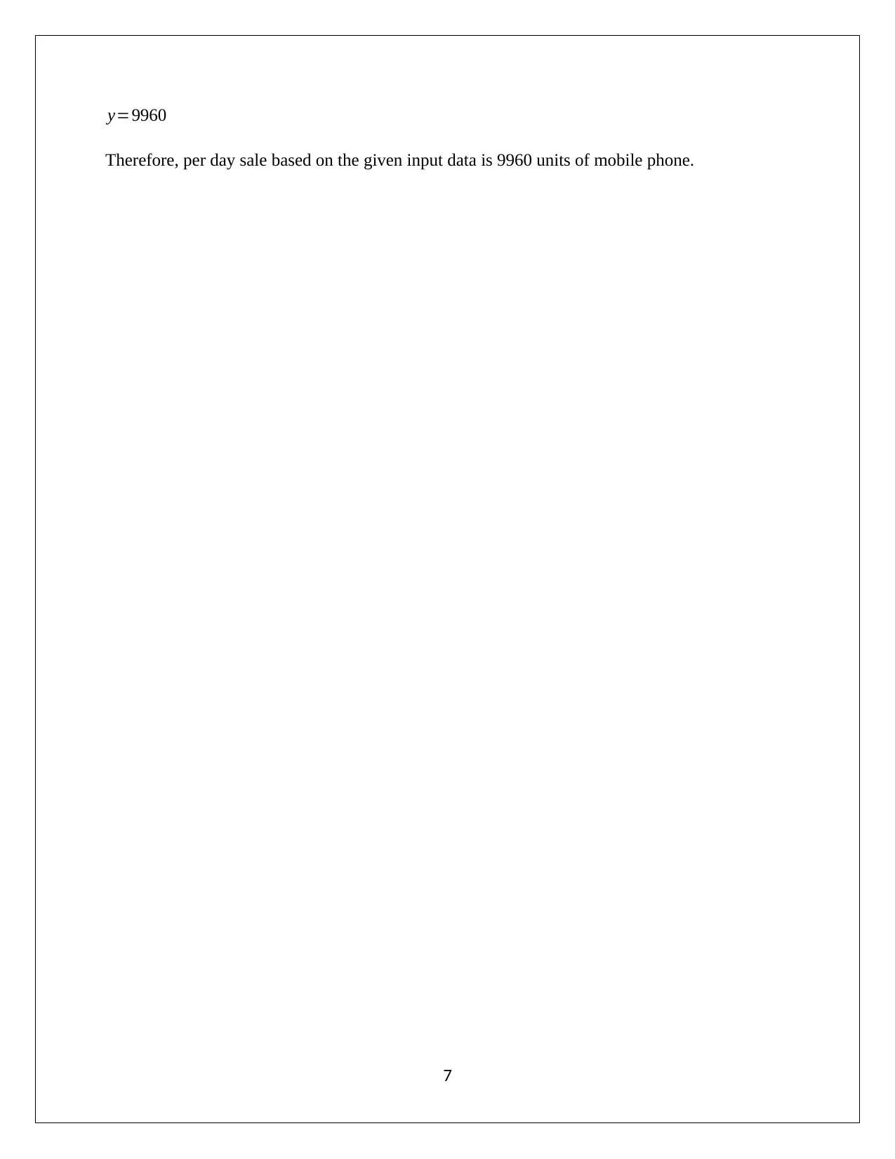
Therefore, per day sale based on the given input data is 9960 units of mobile phone.
7