Analyzing the covariance and correlation between two independent standard Gaussian random variables

This solution explains how to calculate the covariance and correlation between two independent standard Gaussian random variables. It includes step-by-step calculations and examples. Additionally, it clarifies the experimental simulation required to justify the central limit theorem using different sample sizes. The simulation is conducted using R and the results are plotted on histograms with theoretical Gaussian curves.

Question 3
Analytical
Solution
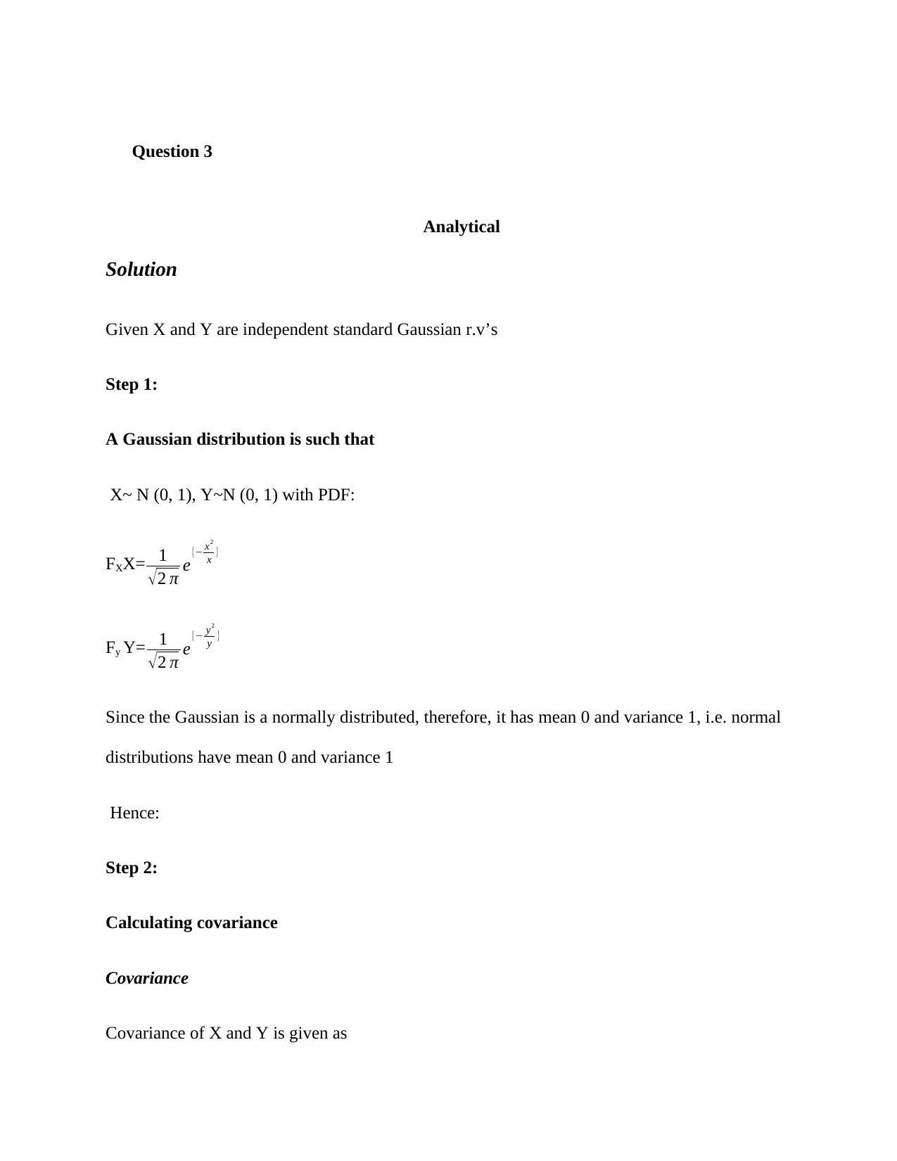
Given X and Y are independent standard Gaussian r.v’s
Step 1:
A Gaussian distribution is such that
X~ N (0, 1), Y~N (0, 1) with PDF:
FXX= 1
√2 π e{− x2
x }
Fy Y= 1
√ 2 π e{− y2
y }
Since the Gaussian is a normally distributed, therefore, it has mean 0 and variance 1, i.e. normal
distributions have mean 0 and variance 1
Hence:
Step 2:
Calculating covariance
Covariance
Covariance of X and Y is given as

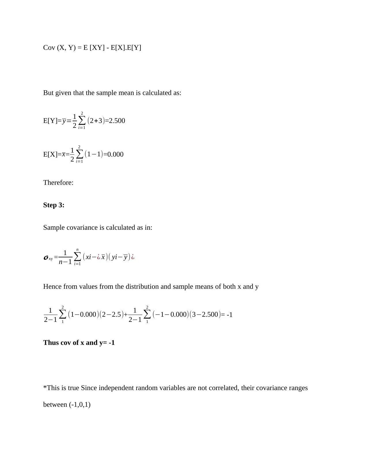
Cov (X, Y) = E [XY] - E[X].E[Y]
But given that the sample mean is calculated as:
E[Y]= y= 1
2 ∑
i=1
2
(2+3)=2.500
E[X]= x= 1
2 ∑
i=1
2
(1−1)=0.000
Therefore:
Step 3:
Sample covariance is calculated as in:
𝓸xy = 1
n−1 ∑
i=1
n
( xi−¿ x )( yi− y ) ¿
Hence from values from the distribution and sample means of both x and y
1
2−1 ∑
1
2
(1−0.000)(2−2.5)+ 1
2−1 ∑
1
2
(−1−0.000)(3−2.500)= -1
Thus cov of x and y= -1
*This is true Since independent random variables are not correlated, their covariance ranges
between (-1,0,1)

Correlation
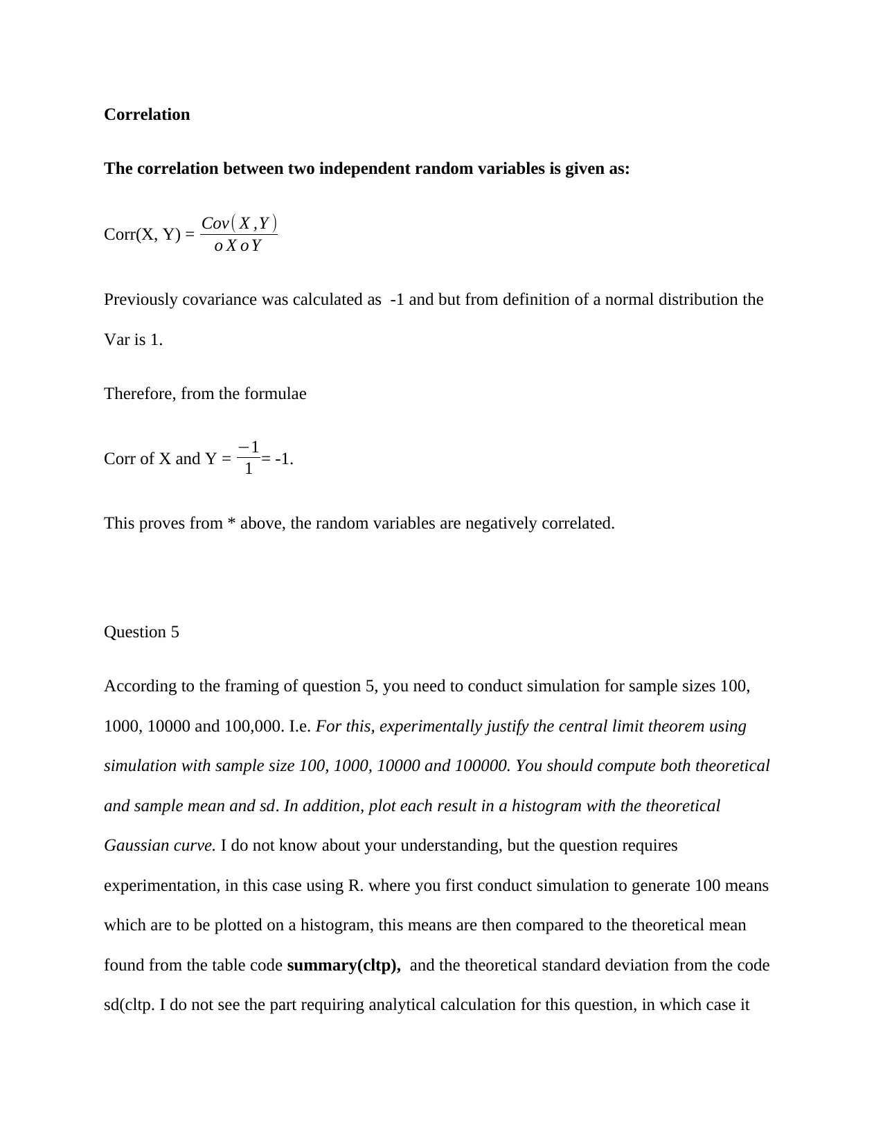
The correlation between two independent random variables is given as:
Corr(X, Y) = Cov( X ,Y )
o X o Y
Previously covariance was calculated as -1 and but from definition of a normal distribution the
Var is 1.
Therefore, from the formulae
Corr of X and Y = −1
1 = -1.
This proves from * above, the random variables are negatively correlated.
Question 5
According to the framing of question 5, you need to conduct simulation for sample sizes 100,
1000, 10000 and 100,000. I.e. For this, experimentally justify the central limit theorem using
simulation with sample size 100, 1000, 10000 and 100000. You should compute both theoretical
and sample mean and sd. In addition, plot each result in a histogram with the theoretical
Gaussian curve. I do not know about your understanding, but the question requires
experimentation, in this case using R. where you first conduct simulation to generate 100 means
which are to be plotted on a histogram, this means are then compared to the theoretical mean
found from the table code summary(cltp), and the theoretical standard deviation from the code
sd(cltp. I do not see the part requiring analytical calculation for this question, in which case it

would be tedious for instance calculating the mean and standard deviations for 100000
simulations analytically. Moreover, that would require us to plot the histogram analytically.
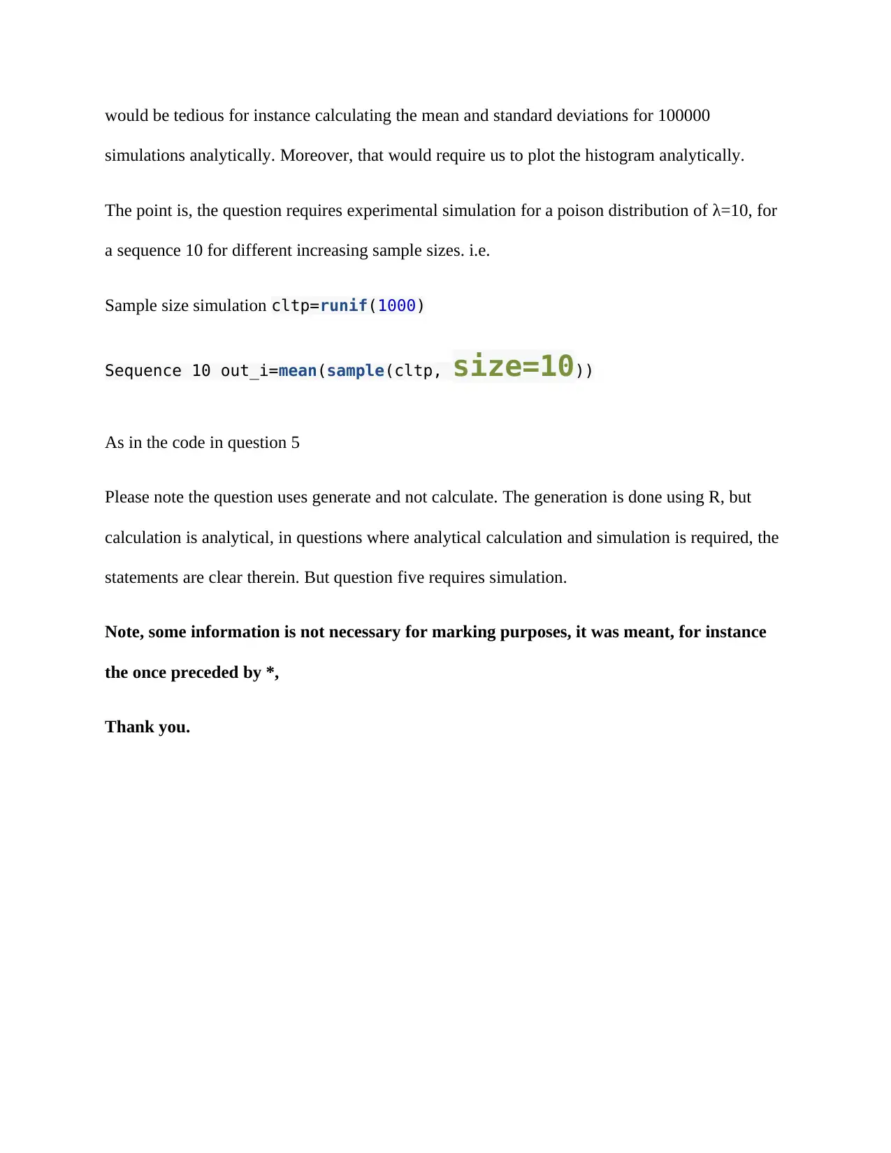
The point is, the question requires experimental simulation for a poison distribution of λ=10, for
a sequence 10 for different increasing sample sizes. i.e.
Sample size simulation cltp=runif(1000)
Sequence 10 out_i=mean(sample(cltp, size=10))
As in the code in question 5
Please note the question uses generate and not calculate. The generation is done using R, but
calculation is analytical, in questions where analytical calculation and simulation is required, the
statements are clear therein. But question five requires simulation.
Note, some information is not necessary for marking purposes, it was meant, for instance
the once preceded by *,
Thank you.