Fruit & Vegetable Intake Comparison

This assignment focuses on comparing the intake of fruits and vegetables between males and females. It utilizes statistical tests such as Levene's Test for Equality of Variances and t-tests to determine if significant differences exist in intake levels. The results are presented along with 95% confidence intervals, allowing for a conclusion about whether female intake is significantly higher than male intake.

Running head: STATISTICS
Statistics
Name of the Student:
Name of the University:
Author’s note:

1STATISTICS
Table of Contents
Introduction:...............................................................................................................................2
Calculation and Analysis:..........................................................................................................2
1) Summary of Categorical variable:...............................................................................2
2) Summary of metric variable:.......................................................................................4
3) Binomial test:.....................................................................................................................7
4) One-sample t-test:........................................................................................................8
5) Independent-samples t-test:.........................................................................................9
References:...............................................................................................................................11

2STATISTICS
Introduction:
The dataset contains 8525 samples of various measures based on health maintaining
processes and scales of lifestyle, exercise and eating habit. The report involves the analysed
data of food habit, exercise level and health quality of randomly selected 2000 variables from
8525 variables.
Drawing of Random Samples:
The researcher had chosen 2000 random variables from 8525 samples by the
following method-
1) Select “Data” option in the menu-bar and then go to “Select cases”.
2) We choose independent variable “ID” and right click on the bullet of random samples
of cases.
3) Then for drawing random samples, we click on the second bullet. We write 2000 in
first box and 8525 in second white box.
4) Lastly, we clicked “Continue” in first drop down-box and then “OK” in second drop
down-box.
5) Our random sample is finally generated.
Calculation and Analysis:
1) Summary of Categorical variable:
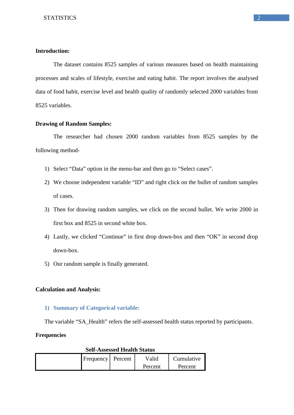
The variable “SA_Health” refers the self-assessed health status reported by participants.
Frequencies
Self-Assessed Health Status
Frequency Percent Valid
Percent
Cumulative
Percent

3STATISTICS
Valid
Excellent 402 20.1 20.1 20.1
Very
Good 710 35.5 35.5 55.6
Good 609 30.5 30.5 86.1
Fair 198 9.9 9.9 96.0
Poor 81 4.1 4.1 100.0
Total 2000 100.0 100.0
Statistics
Self-Assessed Health Status
N Valid 2000
Missing 0
Minimum 1
Maximum 5
Percentiles
25 2.00
50 2.00
75 3.00
Descriptive Statistics
N Rang
e
Minim
um
Maxim
um
Mean Std.
Deviati
on
Varian
ce
Skewness Kurtosis
Statist
ic
Statist
ic
Statisti
c
Statistic Statist
ic
Statisti
c
Statisti
c
Statist
ic
Std.
Err
or
Statist
ic
Std.
Err
or
Self-
Assess
ed
Health
Status
2000 4 1 5 2.42 1.043 1.088 .471 .05
5 -.232 .10
9
Valid
N
(listwis
e)
2000

4STATISTICS
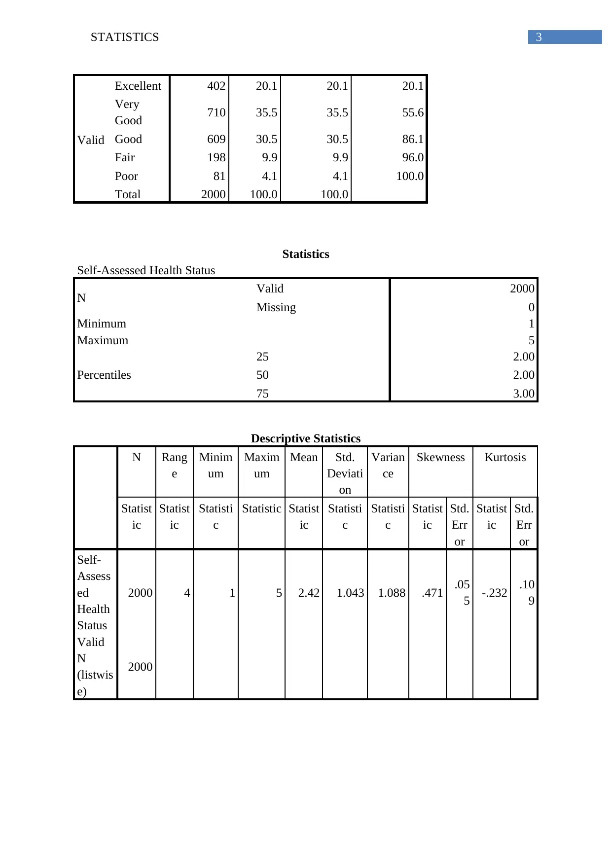
The Frequency table of self-assessed Health Status indicate that among 2000
variables, the health status is “Very Good” for 710 (35.5%) participants followed by “Good”
for 609 (30.5%) participants. The least frequency of health status is “Poor” for 81 (4.1%)
participants. The descriptive statistics indicates that mean of Self Assessed health status is
2.42 and standard deviation is 1.043 (Argyrous, 1997). The mode is “Very Good” (level = 4).
The distribution of self-assessed health-status is positively skewed. The Kurtosis value
indicates that the distribution is “Leptokurtic”. The bar-plot refers that self-assesses health
status has maximum frequency for “Very Good” and minimum frequency for “Poor”
according to the height of bars (Data, 1988). The 1st quartile, median and 3rd quartile values of
the SA_health is 2, 2 and 3. The minimum and maximum values of the SA_health are 1 and
5. The IQR (inter quartile range) is = (3rd quartile – 1st quartile) = (3-2) = 1.

5STATISTICS
2) Summary of metric variable:
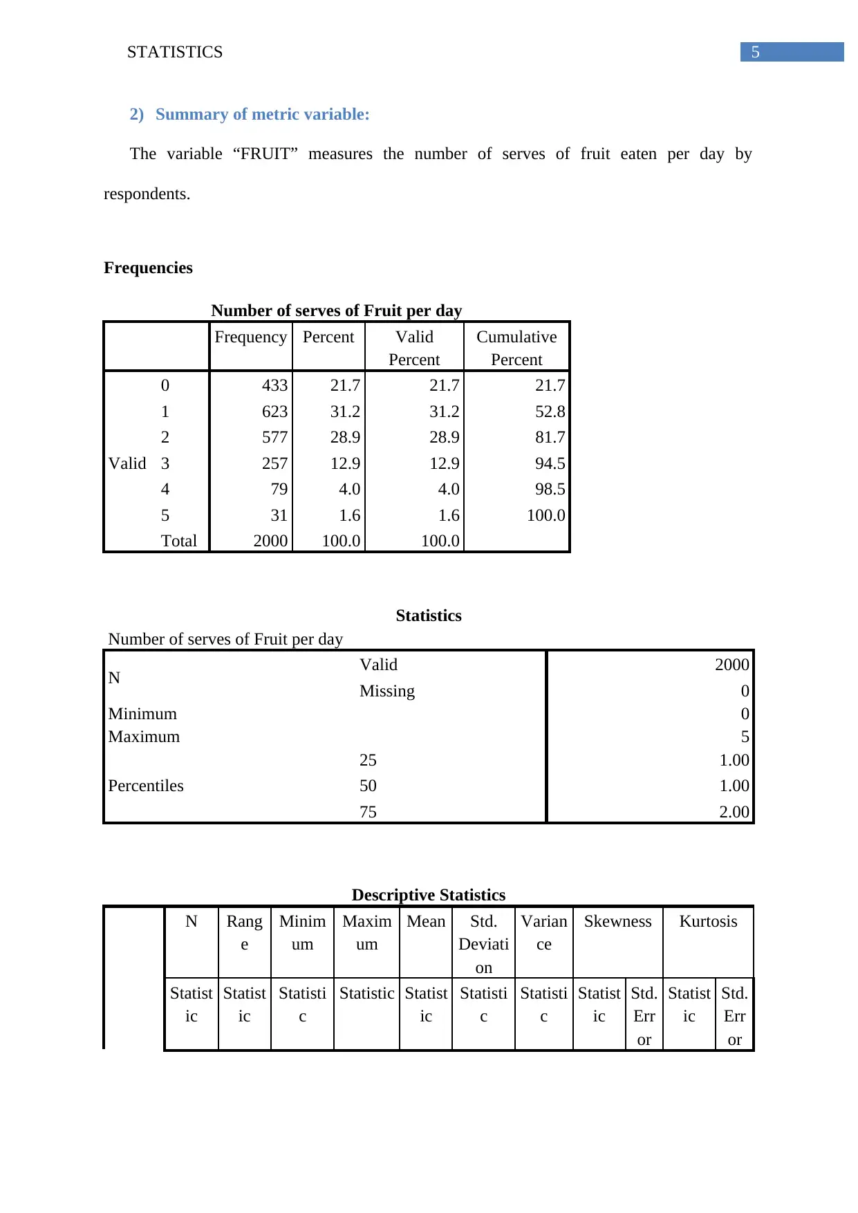
The variable “FRUIT” measures the number of serves of fruit eaten per day by
respondents.
Frequencies
Number of serves of Fruit per day
Frequency Percent Valid
Percent
Cumulative
Percent
Valid
0 433 21.7 21.7 21.7
1 623 31.2 31.2 52.8
2 577 28.9 28.9 81.7
3 257 12.9 12.9 94.5
4 79 4.0 4.0 98.5
5 31 1.6 1.6 100.0
Total 2000 100.0 100.0
Statistics
Number of serves of Fruit per day
N Valid 2000
Missing 0
Minimum 0
Maximum 5
Percentiles
25 1.00
50 1.00
75 2.00
Descriptive Statistics
N Rang
e
Minim
um
Maxim
um
Mean Std.
Deviati
on
Varian
ce
Skewness Kurtosis
Statist
ic
Statist
ic
Statisti
c
Statistic Statist
ic
Statisti
c
Statisti
c
Statist
ic
Std.
Err
or
Statist
ic
Std.
Err
or

6STATISTICS
Numbe
r of
serves
of Fruit
per day
2000 5 0 5 1.51 1.168 1.364 .593 .05
5 .027 .10
9
Valid
N
(listwis
e)
2000
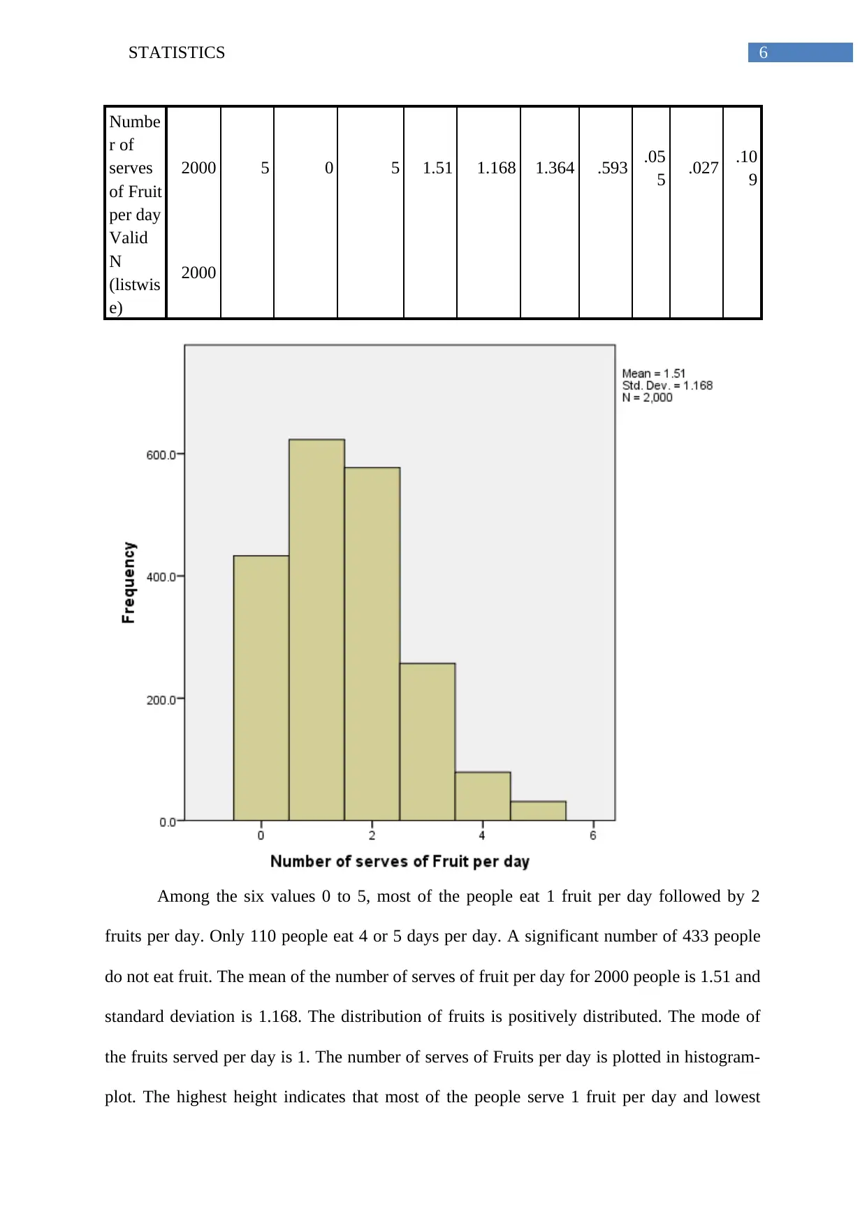
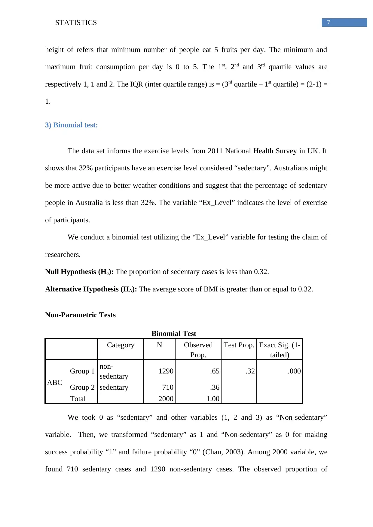
Among the six values 0 to 5, most of the people eat 1 fruit per day followed by 2
fruits per day. Only 110 people eat 4 or 5 days per day. A significant number of 433 people
do not eat fruit. The mean of the number of serves of fruit per day for 2000 people is 1.51 and
standard deviation is 1.168. The distribution of fruits is positively distributed. The mode of
the fruits served per day is 1. The number of serves of Fruits per day is plotted in histogram-
plot. The highest height indicates that most of the people serve 1 fruit per day and lowest

7STATISTICS
height of refers that minimum number of people eat 5 fruits per day. The minimum and
maximum fruit consumption per day is 0 to 5. The 1st, 2nd and 3rd quartile values are
respectively 1, 1 and 2. The IQR (inter quartile range) is = (3rd quartile – 1st quartile) = (2-1) =
1.
3) Binomial test:
The data set informs the exercise levels from 2011 National Health Survey in UK. It
shows that 32% participants have an exercise level considered “sedentary”. Australians might
be more active due to better weather conditions and suggest that the percentage of sedentary
people in Australia is less than 32%. The variable “Ex_Level” indicates the level of exercise
of participants.
We conduct a binomial test utilizing the “Ex_Level” variable for testing the claim of
researchers.
Null Hypothesis (H0): The proportion of sedentary cases is less than 0.32.
Alternative Hypothesis (HA): The average score of BMI is greater than or equal to 0.32.
Non-Parametric Tests
Binomial Test
Category N Observed
Prop.
Test Prop. Exact Sig. (1-
tailed)
ABC
Group 1 non-
sedentary 1290 .65 .32 .000
Group 2 sedentary 710 .36
Total 2000 1.00
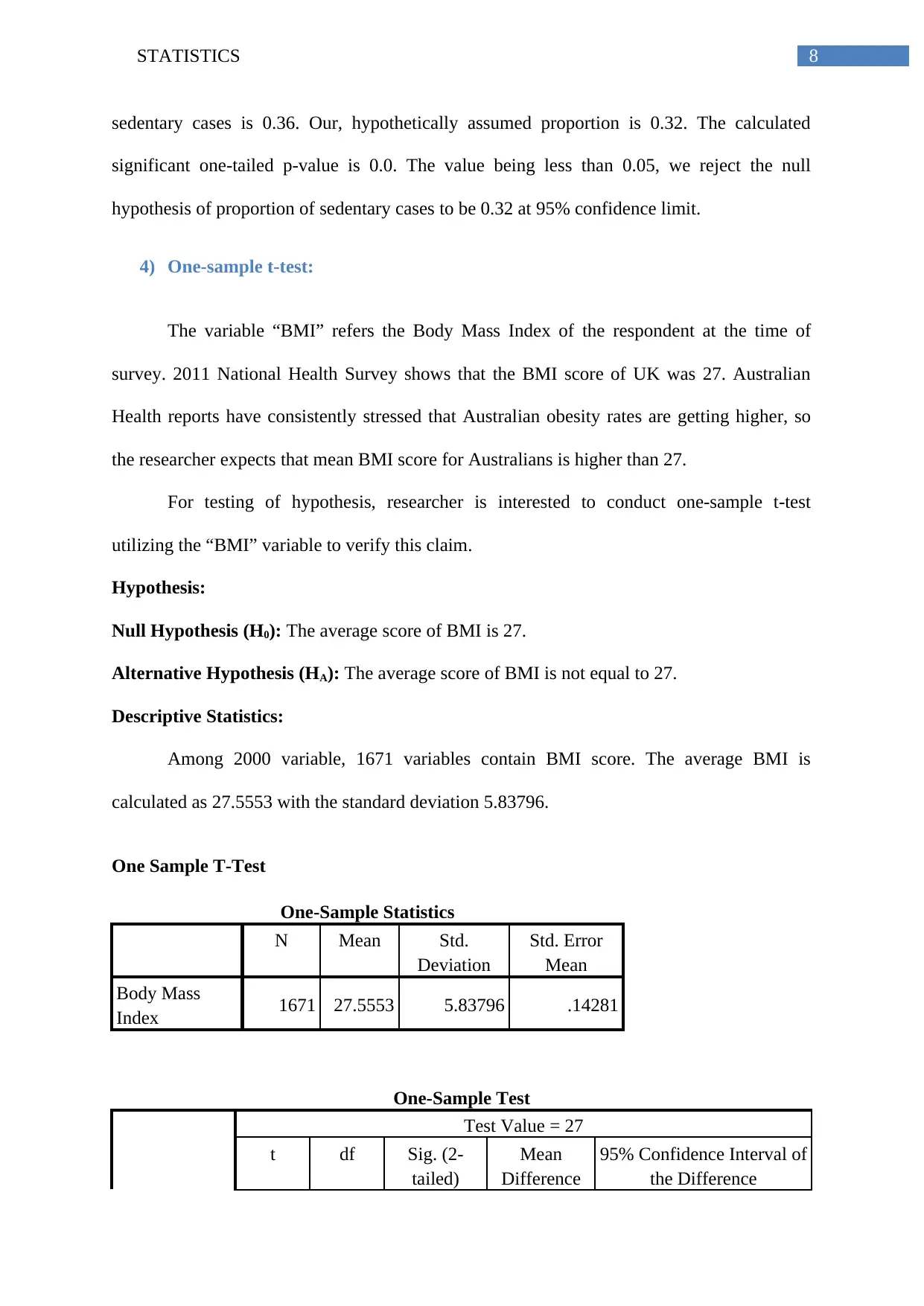
We took 0 as “sedentary” and other variables (1, 2 and 3) as “Non-sedentary”
variable. Then, we transformed “sedentary” as 1 and “Non-sedentary” as 0 for making
success probability “1” and failure probability “0” (Chan, 2003). Among 2000 variable, we
found 710 sedentary cases and 1290 non-sedentary cases. The observed proportion of

8STATISTICS
sedentary cases is 0.36. Our, hypothetically assumed proportion is 0.32. The calculated
significant one-tailed p-value is 0.0. The value being less than 0.05, we reject the null
hypothesis of proportion of sedentary cases to be 0.32 at 95% confidence limit.
4) One-sample t-test:
The variable “BMI” refers the Body Mass Index of the respondent at the time of
survey. 2011 National Health Survey shows that the BMI score of UK was 27. Australian
Health reports have consistently stressed that Australian obesity rates are getting higher, so
the researcher expects that mean BMI score for Australians is higher than 27.
For testing of hypothesis, researcher is interested to conduct one-sample t-test
utilizing the “BMI” variable to verify this claim.
Hypothesis:
Null Hypothesis (H0): The average score of BMI is 27.
Alternative Hypothesis (HA): The average score of BMI is not equal to 27.
Descriptive Statistics:
Among 2000 variable, 1671 variables contain BMI score. The average BMI is
calculated as 27.5553 with the standard deviation 5.83796.
One Sample T-Test
One-Sample Statistics
N Mean Std.
Deviation
Std. Error
Mean
Body Mass
Index 1671 27.5553 5.83796 .14281
One-Sample Test
Test Value = 27
t df Sig. (2-
tailed)
Mean
Difference
95% Confidence Interval of
the Difference

9STATISTICS
Lower Upper
Body Mass
Index 3.888 1670 .000 .55531 .2752 .8354
Inferential Statistics:
The one-sample t-statistic is 3.888 with degrees of freedom 1670. The p-value of this one
sample t-test is 0.0.
Confidential Statistics:
The 95% confidence interval found in the differences of means of BMI indicates that
the lower confidence interval is 0.2752 and upper confidence interval is 0.8354.
Conclusion:
Therefore, we reject the null hypothesis. Hence, the mean of BMI score is not equal to 27
with the probability of 95% (Norušis, 2006).
5) Independent-samples t-test:
As per report, women are being on a diet. The researcher thought that females eat
more fruit and vegetables than males do. For, testing the hypothesis, we conduct an
independent samples t-test utilizing two variables “GENDER” and
“FRUIT_VEG_COMBINED” to test this claim. Among 2000 people, 1026 females eat fruit
and vegetables regularly whereas 974 males eat fruit and vegetables regularly.
Hypotheses:
Null Hypothesis (H0): Females intake equal level of fruit and vegetables as Males
Alternative Hypothesis (HA): Females intake more fruit and vegetables as Females
Descriptive Statistics:
Among 2000 people, 974 males and 1026 females intake fruit & vegetable combined
per day. The average fruit & vegetables for males and females are 3.71 and 4.08.

10STATISTICS
Independent sample T-Test
Group Statistics
Gender N Mean Std.
Deviation
Std. Error
Mean
Fruit & Vegetable
Intake combined [per
day]
Male 974 3.71 2.457 .079
Female 1026 4.08 2.397 .075
Independent Samples Test
Levene's
Test for
Equality
of
Variance
s
t-test for Equality of Means
F Sig. t df Sig.
(2-
tailed
)
Mean
Differenc
e
Std. Error
Differenc
e
95%
Confidence
Interval of
the
Difference
Lowe
r
Uppe
r
Fruit &
Vegetabl
e Intake
combine
d [per
day]
Equal
variance
s
assumed
.25
6
.61
3
-
3.34
9
1998 .001 -.363 .109 -.576 -.151
Equal
variance
s not
assumed
-
3.34
6
1986.33
3 .001 -.363 .109 -.577 -.150
Inferential Statistics:
The Levene’s test for equality of variances indicates F-statistic = 0.256 with
significant p-values 0.613 (Mehta and Patel, 2010). Therefore, we can conclude that
variances are not equal for male and female intake level of fruits and vegetables. The t-
statistic of equality of means indicate that t-values for equal variance (-3.349) and unequal

11STATISTICS
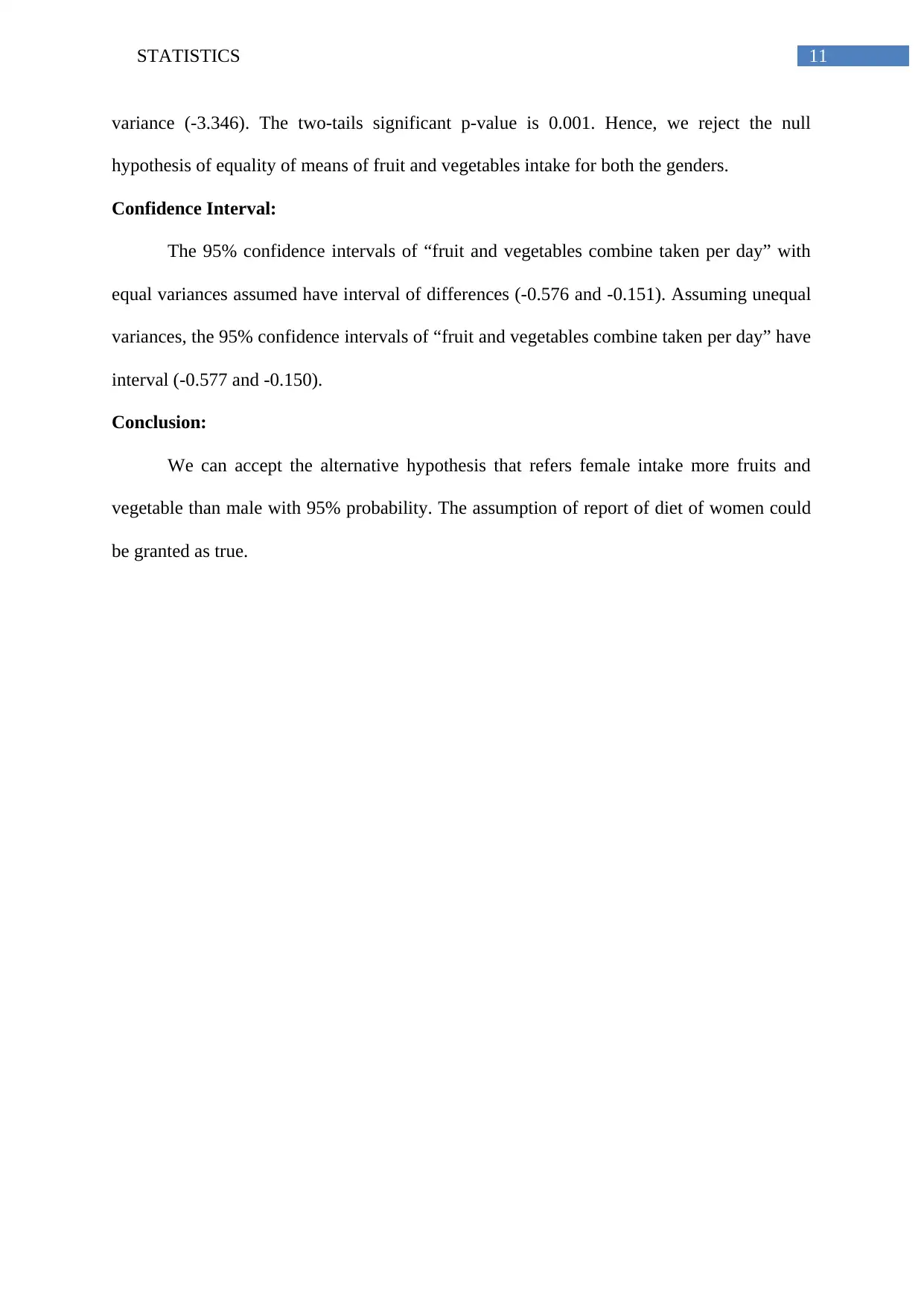
variance (-3.346). The two-tails significant p-value is 0.001. Hence, we reject the null
hypothesis of equality of means of fruit and vegetables intake for both the genders.
Confidence Interval:
The 95% confidence intervals of “fruit and vegetables combine taken per day” with
equal variances assumed have interval of differences (-0.576 and -0.151). Assuming unequal
variances, the 95% confidence intervals of “fruit and vegetables combine taken per day” have
interval (-0.577 and -0.150).
Conclusion:
We can accept the alternative hypothesis that refers female intake more fruits and
vegetable than male with 95% probability. The assumption of report of diet of women could
be granted as true.

12STATISTICS
References:
Argyrous, G. (1997). Descriptive statistics on SPSS. In Statistics for Social Research (pp. 60-
78). Palgrave, London.
Chan, Y. H. (2003). Biostatistics 102: quantitative data–parametric & non-parametric
tests. blood pressure, 140(24.08), 79-00.
Data, C. E. (1988). Basic statistical concepts.
Mehta, C. R., & Patel, N. R. (2010). IBM SPSS exact tests. SPSS Inc., Cambridge, MA.
Norušis, M. J. (2006). SPSS 14.0 guide to data analysis. Upper Saddle River, NJ: Prentice
Hall.
Muijs, D. (2010). Doing quantitative research in education with SPSS. Sage.

13STATISTICS