Data Analysis Report of Health and Population Statistics of East Asian and Pacific Countries

This report analyses the health and population statistics of East Asian and Pacific countries from 2001 to 2015. The report includes one-variable and two-variable analysis, clustering, and linear regression. The data has been collected from World Bank.

Data analysis report of the health and population statistics of East Asian and Pacific countries
Name of the Student

Table of Contents
1 Introduction..................................................................................................................................1
1.1 Authorisation and Purpose...............................................................................................1
Limitations...................................................................................................................................1
Scope............................................................................................................................................1
Methodology...............................................................................................................................1
2 Data Setup....................................................................................................................................1
3 Exploratory Data Analysis.............................................................................................................2
3.1 One Variable Analysis................................................................................................................2
3.1.1 One Variable Analysis – 1.......................................................................................................2
3.1.2 One Variable Analysis – 2.......................................................................................................3
3.1.3 One Variable Analysis – 3.......................................................................................................6
3.2 Two-variable analysis.................................................................................................................7
3.2.1 Two-variable analysis 1...........................................................................................................7
3.2.2 Two-variable analysis 2...........................................................................................................8
4 Advanced analysis.......................................................................................................................10
4.1 Clustering.................................................................................................................................10
4.1.1 Brief explanation of k-means and clustering........................................................................10
4.1.2 Clustering Analysis................................................................................................................11
4.2 Linear regression......................................................................................................................12
4.2.1 Brief definition of linear regression......................................................................................12
4.2.2 Linear Regression 1...............................................................................................................13
4.2.3 Linear Regression 2...............................................................................................................14
5 Conclusion...................................................................................................................................16
6 Reflection....................................................................................................................................16
Reference.......................................................................................................................................17
Page | ii

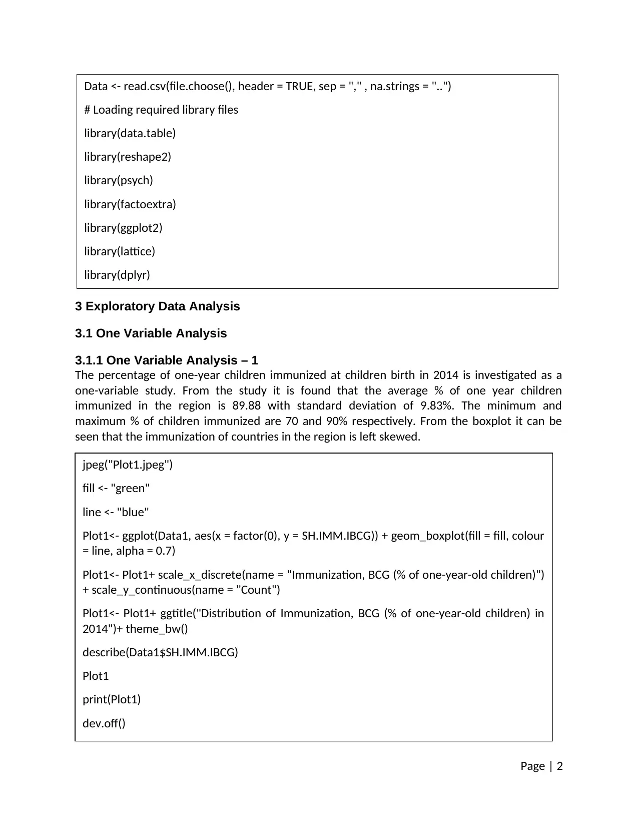
1 Introduction
1.1 Authorisation and Purpose
The purpose of the present study is to analyse the health of East Asia and Pacific region with
reference to the period of 2001 to 2015. The data has been collected for World Bank. The
analysis of the data has implications for governments and planners. Improvements in the health
of the region can be initiated through the present study.
Limitations
The information provided for the present investigation pertains to the region of East Asia and
Pacific. The data has been taken from World Bank. In addition, the time period chosen for the
study is from 2001 to 2015.
The analysis is limited to the region of East Asia and Pacific only.
Scope
The data for the present study is replete with information related to the health of the region.
There are 26 attributes in the study with countries of East Asia and Pacific region. In addition,
the study present information on the attributes for the period of 2001 to 2015. However, the
data derived from the world bank has lots of missing data.
The analysis of the data is done through statistical analysis and interpretation of graphs. In the
first stage the data has been studied through three one-variable analyses. In the second stage
two-variable analysis is used. Next we analyse the information through k-means clustering.
Finally, relation between two attributes is studied through linear regression.
Methodology
For the analysis of the health of the East Asia and Pacific region quantitative information for the
period of 2001 to 2015 is studied. The information for the study has been gathered from World
Bank.
2 Data Setup
Before the analysis of the data can take place the data file needs to be loaded into the “R”
program. When the first line of Code is run a pop-up window opens. The user is requested to
input the location of the data file. Moreover, when the file is loaded into the “R” program the
first row is taken as the header. In addition, it was found that there are many missing values in
the “CSV” file, these are denoted as missing is the first line of code.
The second stage of the data analysis provides information to “R program” to load library files.
Library files are necessary to carry out different statistical tests and also to produce charts and
graphs.

3 Exploratory Data Analysis
3.1 One Variable Analysis
3.1.1 One Variable Analysis – 1
The percentage of one-year children immunized at children birth in 2014 is investigated as a
one-variable study. From the study it is found that the average % of one year children
immunized in the region is 89.88 with standard deviation of 9.83%. The minimum and
maximum % of children immunized are 70 and 90% respectively. From the boxplot it can be
seen that the immunization of countries in the region is left skewed.
Page | 2
jpeg("Plot1.jpeg")
fill <- "green"
line <- "blue"
Plot1<- ggplot(Data1, aes(x = factor(0), y = SH.IMM.IBCG)) + geom_boxplot(fill = fill, colour
= line, alpha = 0.7)
Plot1<- Plot1+ scale_x_discrete(name = "Immunization, BCG (% of one-year-old children)")
+ scale_y_continuous(name = "Count")
Plot1<- Plot1+ ggtitle("Distribution of Immunization, BCG (% of one-year-old children) in
2014")+ theme_bw()
describe(Data1$SH.IMM.IBCG)
Plot1
print(Plot1)
dev.off()
Data <- read.csv(file.choose(), header = TRUE, sep = "," , na.strings = "..")
# Loading required library files
library(data.table)
library(reshape2)
library(psych)
library(factoextra)
library(ggplot2)
library(lattice)
library(dplyr)

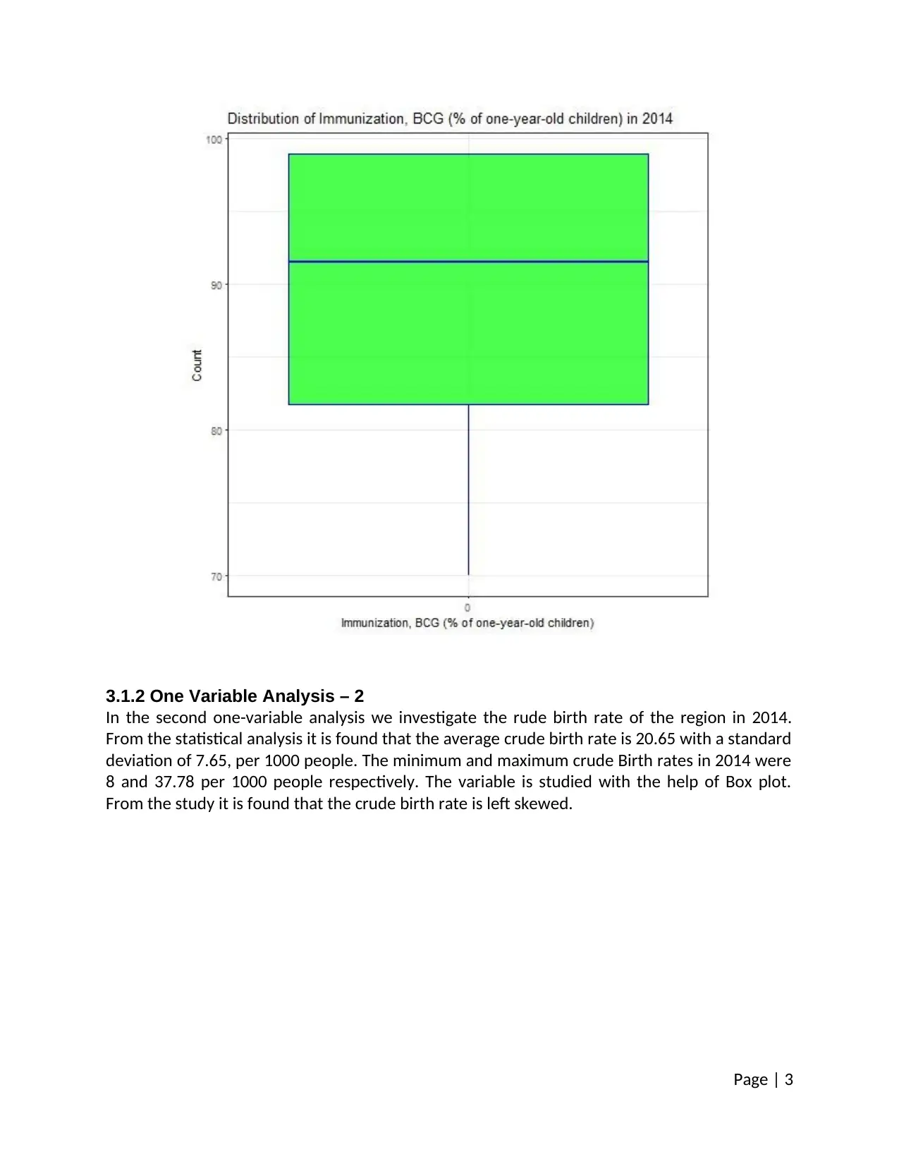
3.1.2 One Variable Analysis – 2
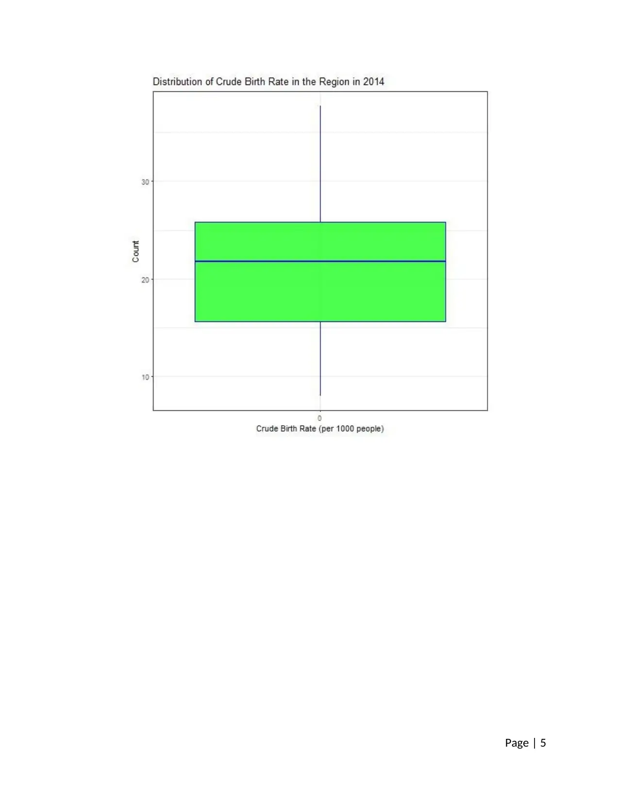
In the second one-variable analysis we investigate the rude birth rate of the region in 2014.
From the statistical analysis it is found that the average crude birth rate is 20.65 with a standard
deviation of 7.65, per 1000 people. The minimum and maximum crude Birth rates in 2014 were
8 and 37.78 per 1000 people respectively. The variable is studied with the help of Box plot.
From the study it is found that the crude birth rate is left skewed.
Page | 3

Page | 4
jpeg("Plot2.jpeg")
fill <- "green"
line <- "blue"
Plot2 <- ggplot(Data1, aes(x = factor(0), y = SP.DYN.CBRT.IN)) + geom_boxplot(fill = fill,
colour = line, alpha = 0.7)
Plot2 <- Plot2 + scale_x_discrete(name = "Crude Birth Rate (per 1000 people)") +
scale_y_continuous(name = "Count")
Plot2 <- Plot2 + ggtitle("Distribution of Crude Birth Rate in the Region in 2014")+
theme_bw()
describe(Data1$SP.DYN.CBRT.IN)
Plot2
print(Plot2)
dev.off()

Page | 5

3.1.3 One Variable Analysis – 3
Histogram is a useful depiction of a one-variable. The rate of immunization is studies using
histogram. From the plotted histogram it can be seen that most of the countries of the region
have a very high level of immunization against BCG.
Page | 6
jpeg("Plot3.jpeg")
Plot3 <- ggplot(Data1, aes(x = SH.IMM.IBCG))+ geom_histogram(binwidth = 2,col="blue",
fill="green")
Plot3 <- Plot3 + scale_x_continuous("Immunization, BCG (% of one-year-old children)") +
scale_y_continuous("Count")+theme_bw()
Plot3 <- Plot3 + ggtitle("Distribution of Immunization, BCG (% of one-year-old children) in 2014")
Plot3
print(Plot3)
dev.off()

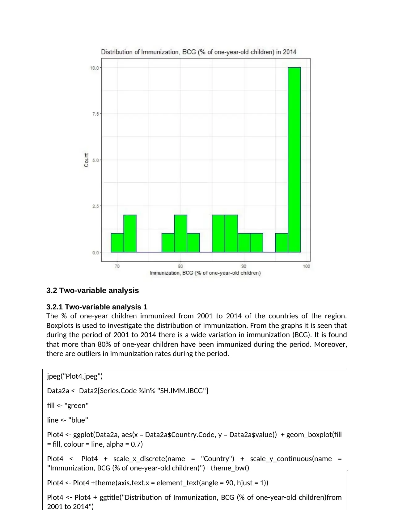
3.2 Two-variable analysis
3.2.1 Two-variable analysis 1
The % of one-year children immunized from 2001 to 2014 of the countries of the region.
Boxplots is used to investigate the distribution of immunization. From the graphs it is seen that
during the period of 2001 to 2014 there is a wide variation in immunization (BCG). It is found
that more than 80% of one-year children have been immunized during the period. Moreover,
there are outliers in immunization rates during the period.
Page | 7
jpeg("Plot4.jpeg")
Data2a <- Data2[Series.Code %in% "SH.IMM.IBCG"]
fill <- "green"
line <- "blue"
Plot4 <- ggplot(Data2a, aes(x = Data2a$Country.Code, y = Data2a$value)) + geom_boxplot(fill
= fill, colour = line, alpha = 0.7)
Plot4 <- Plot4 + scale_x_discrete(name = "Country") + scale_y_continuous(name =
"Immunization, BCG (% of one-year-old children)")+ theme_bw()
Plot4 <- Plot4 +theme(axis.text.x = element_text(angle = 90, hjust = 1))
Plot4 <- Plot4 + ggtitle("Distribution of Immunization, BCG (% of one-year-old children)from
2001 to 2014")

Page | 8

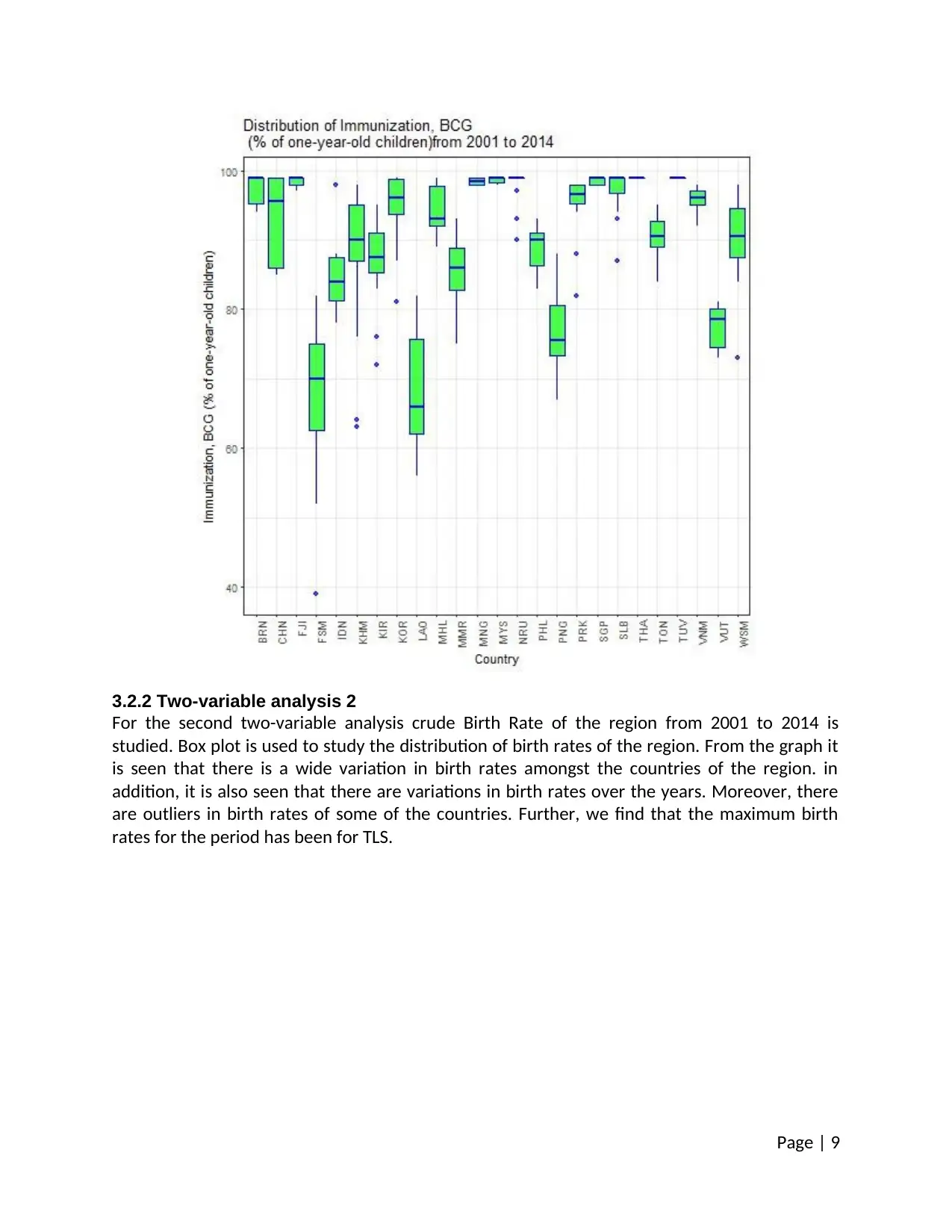
3.2.2 Two-variable analysis 2
For the second two-variable analysis crude Birth Rate of the region from 2001 to 2014 is
studied. Box plot is used to study the distribution of birth rates of the region. From the graph it
is seen that there is a wide variation in birth rates amongst the countries of the region. in
addition, it is also seen that there are variations in birth rates over the years. Moreover, there
are outliers in birth rates of some of the countries. Further, we find that the maximum birth
rates for the period has been for TLS.
Page | 9

Page | 10
jpeg("Plot5.jpeg")
Data2b <- Data2[Series.Code %in% "SP.DYN.CBRT.IN"]
fill <- "green"
line <- "blue"
Plot5 <- ggplot(Data2b, aes(x = Data2b$Country.Code, y = Data2b$value)) + geom_boxplot(fill =
fill, colour = line, alpha = 0.7)
Plot5 <- Plot5 + scale_x_discrete(name = "Country") + scale_y_continuous(name = "Crude Birth
Rate (per 1000 people)")+ theme_bw()
Plot5 <- Plot5 +theme(axis.text.x = element_text(angle = 90, hjust = 1)) + ggtitle("Distribution of
Crude Birth Rate from 2001 to 2014")
Plot5
print(Plot5)
dev.off()

4 Advanced analysis
4.1 Clustering
4.1.1 Brief explanation of k-means and clustering
The process of clustering involves the segregation of data into groups. The centre of a group is a
representative of the group. There are different methods of clustering. K-means clustering
involves the use of centroids for segregating the groups (Oleiwi 2016). Centroids are first
chosen and then the data points are assigned to the centroid which is nearest to the value of
the data. Whenever a data point is added the mean of the group is calculated and the centroid
is moved according to the value. The process is repeated till all the data points are utilised
(Witten et al., 2016).
Page | 11

4.1.2 Clustering Analysis
Page | 12
jpeg("Plot6.jpeg")
Data4 <- filter(Data, Series.Code %in% c("SP.DYN.CBRT.IN","SH.IMM.IBCG"))
Data4 <- subset(Data4, select = -(X2015..YR2015.))
Data4 <- melt(Data4, Series.Code = c("Series.Code","Country.Name","Country.Code"))
Data4 <- dcast(Data4, formula = Country.Code ~ Series.Code, mean)
Data4 <- na.omit(Data4)
Data4
grpdata <- kmeans(Data4[,c("SP.DYN.CBRT.IN","SH.IMM.IBCG")],centers = 3, nstart = 10)
grpdata
o = order(grpdata$cluster)
data.frame(Data4$Country.Code[o], grpdata$cluster[o])
Plot6 <- plot(Data4$SP.DYN.CBRT.IN, Data4$SH.IMM.IBCG, type="n", xlim=c(8,50),
xlab="Crude Birth Rate", ylab="Immunization")+ text(x=Data4$SP.DYN.CBRT.IN,
y=Data4$SH.IMM.IBCG, labels=Data4$Country.Code,col=grpdata$cluster+1)
print(Plot6)
dev.off()

The crude birth rate of the region in 2014 is clustered with the immunization rate. From scaling it is
found that the countries can best grouped when there are three clusters. From the above chart it is
found that there are three groups –
Low crude birth rate and High level of immunization
High Birth rate but Low level of immunization
High Crude Birth Rate and Average level of immunization
4.2 Linear regression
4.2.1 Brief definition of linear regression
The relation between response and predictor variable is modelled with the help of linear
regression. The predictor variable in a regression analysis is used to forecast changes which
might take place in the response variable (Theobald and Freeman 2014). The relation between
predictor and response variable is shown as:
Page | 13

Y =mX +C
In the above equation “Y” is the response variable and “X” is the predictor variable (Herkenhoff
and Fogli 2013). The above equation also demonstrates that for each unit change in value of
“X” the values of “Y” changes “m” times.
4.2.2 Linear Regression 1
The relation between crude birth rate and immunization for the year 2014 was investigated in
the first regression analysis. It was assumed that with increase in child birth rates of the region
there would be a corresponding increase in immunization rate also. Immunization of children
are necessary so as to increase their immunity level and thus increase their resistance to
diseases. However, the analysis shows that with increase in child birth rate there has been a
decrease in immunization rate.
The immunization is predicted as:
Immunization = 106.1735 – 0.7603*Child Birth Rate
Page | 14
jpeg("Plot7.jpeg")
Plot7 <- lm(formula = SH.IMM.IBCG ~ SP.DYN.CBRT.IN, data = Data3)
summary(Plot7)
Plot7 <- ggplot(Data3, aes(x = SP.DYN.CBRT.IN, y=SH.IMM.IBCG)) + geom_point(shape=4)
Plot7 <- Plot7 + scale_x_continuous(name = "Crude Birth Rate") + scale_y_continuous(name
= "Child Immunization Rate")+ geom_smooth(method=lm)
Plot7 <- Plot7 + theme_bw()+ ggtitle("Relation of Crude Birth Rate to Immunization Rate in
2014")
print(Plot7)
dev.off()

4.2.3 Linear Regression 2
The relation between crude birth rate and school enrolment for the year 2014 was investigated
in the first regression analysis. It was assumed that with increase in child birth rates of the
region there would be a corresponding increase in primary school enrolment of the children.
The increase in primary schooling would mean an increase in education level of the children of
the region. The analysis shows that with increase in child birth rate there is a corresponding
increase in enrolment of children in primary schooling.
The enrolment is predicted as:
Enrolment = 0.5367*Child Birth Rate – 36.3354
Page | 15

Page | 16
jpeg("Plot8.jpeg")
Plot8 <- lm(formula = SP.DYN.CBRT.IN ~ SE.PRM.ENRR, data = Data3)
summary(Plot8)
Plot8 <- ggplot(Data3, aes(x = SP.DYN.CBRT.IN, y=SE.PRM.ENRR)) + geom_point(shape=4)
Plot8 <- Plot8 + scale_x_continuous(name = "Crude Birth Rate") +
scale_y_continuous(name = "School enrollment, primary (% gross)")+
geom_smooth(method=lm)
Plot8 <- Plot8 + theme_bw()+ ggtitle("Relation of Crude Birth Rate to School Enrolement
in 2014")
print(Plot8)
dev.off()

5 Conclusion
The investigation into the health statistics analysis of the region provided important insights.
From the analysis it is found that for most of the countries there is a high level of immunization
in 2014. Moreover, the crude Birth rate in 2014 had a lot of variations. From two-variable
analysis the immunization distribution is found over the last 14 years. From the study it can be
seen that even though for most of the countries there has been a high level of immunization for
some countries the immunization level is low. Moreover, there are wide variations in crude
birth rate over the last 14 years. Further, in the clustering process it is found that the countries
of the region can be segregated into three groups based on crude birth rate and immunization
level. Additionally, it is found that there is increase in primary school enrolment with increase in
crude birth rate. Conversely it is also found that there is a decrease in immunization level with
increase in crude birth rates.
6 Reflection
The investigation into the health statistics of East Asia and Pacific Region was made interesting
by the fact that the variables to be used were in attribute form. Moreover, there was presence
of missing data. Through the study we could find the variations in birth rates and immunization
levels of the region. In addition, we came to know that there has been a growth in primary
enrolment of the region. However, it was a shock to know from the analysis that there is
decline in immunization levels with increase in Crude Birth Rates.
Page | 17

Reference
Herkenhoff, L. and Fogli, J., 2013. Simple Linear Regression. In Applied Statistics for Business
and Management using Microsoft Excel (pp. 221-247). Springer, New York, NY.
Oleiwi, W.K., 2016. Using the Fuzzy Logic to Find Optimal Centers of Clusters of K-means.
International Journal of Electrical and Computer Engineering, 6(6), p.3068.
Theobald, R. and Freeman, S., 2014. Is it the intervention or the students? Using linear
regression to control for student characteristics in undergraduate STEM education research.
CBE-Life Sciences Education, 13(1), pp.41-48.
Witten, I.H., Frank, E., Hall, M.A. and Pal, C.J., 2016. Data Mining: Practical machine learning
tools and techniques. Morgan Kaufmann.
Page | 18